Preventive Maintenance and the Cost Per Unit Time Equation

Components that wear out are candidates for preventive maintenance. When the cost to replace a component before it fails is less than the cost to replace the component after it fails, it makes sense to maintain the component preventively. The optimum preventive maintenance time can be found using the Weibull++, BlockSim and RCM++ software packages from ReliaSoft. These methods are based on the cost per unit time to maintain the component, and they are presented in this article.

Consider a non-repairable component with a failure rate behavior that is independent of the age of the system in which it is installed. The component has a life described by a Weibull distribution with β = 3 and η = 150 days. It will cost $8 each time the component is replaced after it fails (corrective maintenance), while it will cost $2 to replace the component before it fails (preventive maintenance). It is the job of the reliability engineer to determine the optimum preventive maintenance time for the component.

The optimum solution to this problem will be to choose the preventive maintenance time that minimizes the cost per unit time. The equation describing cost per unit time is as follows:

where CPUT is the cost per unit time, CP is the cost of a planned (preventive) replacement, CU is the cost of an unplanned (corrective) replacement, R(t) is the reliability function for the component and t is the preventive maintenance time. Note that the costs used for this model can be due to a variety of causes, which include things such as monetary cost to replace the component, cost of diminished company reputation and cost of lawsuits associated with failures. The numerator of this expression represents the average cost for a single replacement. It is the costs of preventive and corrective maintenance actions weighted by the probabilities that the component will survive or not survive the preventive maintenance interval. The denominator of this expression represents the average time until a single component is replaced. The expression in the denominator is not easy to explain as it is written. However, if the denominator is integrated by parts, the cost per unit time equation becomes:

where f(t) is the probability density function (pdf) for the component. The first term is the replacement time multiplied by the probability that the component will survive until the scheduled maintenance. The second term is the expected value of the pdf on the interval from 0 to the replacement time. In other words, it represents the expected failure time of the components that fail before the scheduled maintenance time, weighted by the percentage of the components that do not survive until the scheduled preventive maintenance action.

In order to determine the lowest cost per unit time for this component, the time, t, must be chosen to minimize the CPUT equation. This can be accomplished by taking the derivative of the CPUT equation, setting this derivative to zero, and solving for t. The mathematical details are beyond the scope of this article.

One approach to solving this problem is to use the Optimum Replacement report template in Weibull++. First, the components failure rate behavior must be defined in a Standard Folio. The analyst could use a Folio containing component failure times and calculate the parameters of the pdf for the component, but for the purpose of this example, we will assume that the parameters describing the failure distribution of the component are known from a previous analysis. The analyst creates a new times-to-failure Folio but does not enter any data in the Data Sheet. When she clicks Calculate, the Parameter Input window appears, allowing her to enter the parameters of the distribution, as shown in Figure 1.

Figure 1: The Parameters of the pdf (β = 3 and η = 150 hours) Are Prescribed

When the analyst clicks OK, the parameters entered in the dialog box appear in the Folio's Control Panel, as shown in Figure 2.

Figure 2: The Weibull++ Folio Containing the Parameters for the Component

Next, the analyst chooses Project > Add Report and the Report Wizard opens. In order to link the report to the Data Sheet with the components parameters, the analyst clicks Select and selects the Data Sheet in the Select Folio/Data Sheet window, as shown in Figure 3.

Figure 3: The Data Sheet Is Linked to the Report

The analyst then selects the Based on an existing Template check box and chooses the Optimum Replacement template, as shown in Figure 4.

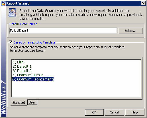
Figure 4: Choosing the Optimum Replacement Report Template

When the analyst clicks OK, the report shown in Figure 5 is created.

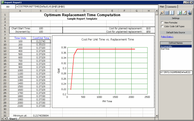
Figure 5: The Default Optimum Replacement Report

The cost per unit time values in column B are computed using the formula for CPUT given above. Note that clicking a cell in column B (for example, consider cell B9) displays an equation using the built-in function COSTPERUNITTIME in the data entry box at the top of the report. The arguments for this function are:

• Default, which contains either a link to or the name of the data sheet containing the components parameters.
• A9, which contains the time at which the cost per unit time is computed.
• H5 and H6, which contain the costs for preventive and corrective maintenance actions, respectively.

The report displays cost per unit time values for times ranging from 100 to 2100 days using the default settings. However, since the characteristic life, or the time by which 63.2% of the components are expected to fail, is 150 days, the analyst must reduce the time values to capture the optimum replacement time. In addition, the default costs in the report are not the actual costs for the component. After the analyst alters the top rows of the report to reflect these changes, the report appears as shown in Figure 6.

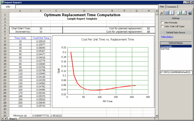
Figure 6: Using the Optimum Replacement Report in Weibull++ to Determine Optimum Preventive Maintenance Time

The optimum preventive maintenance time and corresponding cost per unit time are shown in both the table and graphically. The optimum preventive maintenance time for this scenario is around 80 days and the corresponding cost per unit time is 3.69 per day.

A second way to determine the optimum maintenance time for a non-repairable component is to use the Optimum Replacement tool in BlockSim. The analyst creates a single block to represent the component, then double-clicks the block to open the Block Properties window. On the Reliability tab, she enters the parameters of the distribution, as shown in Figure 7, and then clicks OK.

Figure 7: Assigning the Parameters of the pdf to the Block

The analyst then right-clicks the block and chooses Optimum Replacement in the shortcut menu that appears. She enters the planned and unplanned replacement costs and clicks Calculate to obtain the results shown in Figure 8.

Figure 8: Using the Optimum Replacement Tool in BlockSim to Determine Preventive Maintenance Time

A third method to determine the optimum preventive maintenance time is to use the Optimum Maintenance tool in RCM++. The optimum preventive maintenance interval in RCM++ is calculated at the task level, using information specified for the task and for the cause.

The analyst double-clicks the cause of interest to open the Cause Properties window. On the Probablility page, she enters the parameters of the Weibull distribution, as shown in Figure 9.

Figure 9: Entering the Probability Parameters for the Cause

She enters the costs associated with corrective maintenance on the Corrective Maintenance page, as shown in Figure 10.

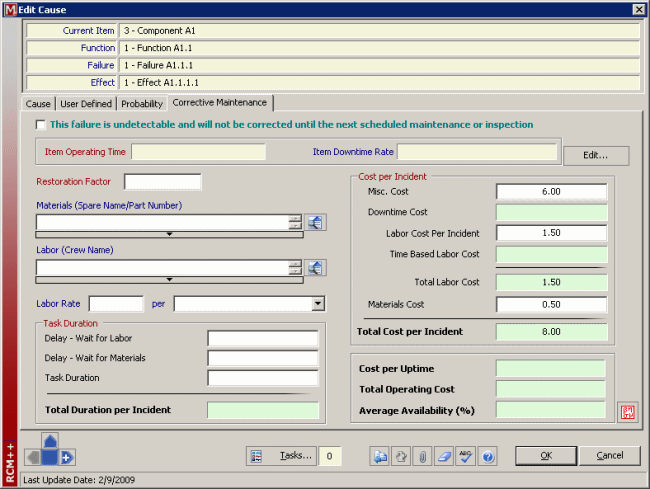
Figure 10: Entering the Corrective Maintenance Costs

Next, the analyst clicks the Tasks button to open the Task Manager, where she clicks the Add Task button. In the Task Properties window that appears, she will set up the replacements. She enters a Task Name, chooses Repair/Replace in the Type field, chooses Day in the Units field for the Assigned Interval and verifies that the Assigned Interval is based on Item Age, as shown in Figure 11.

Figure 11: Defining a New Task

To assign costs associated with the preventive maintenance action, the analyst goes to the PM Resources page of the Task Properties window. She then enters the costs, as shown in Figure 12.

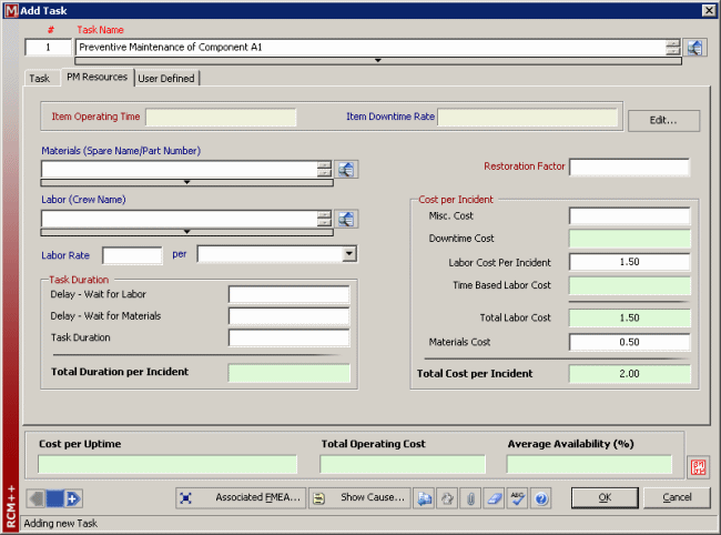
Figure 12: Entering the Preventive Maintenance Costs

The analyst returns to the Task page and clicks the Calculate Optimum button. The Calculated Optimum Interval window shown in Figure 13 appears and prompts her to choose how the calculated optimum interval will be used. This gives the analyst the option to use this calculated value as the assigned interval for the task or, if desired, to store it as a proposed interval and to round up or down, according to her needs, for the actual assigned interval. In this case, she selects Set as Assigned Interval and clicks OK.

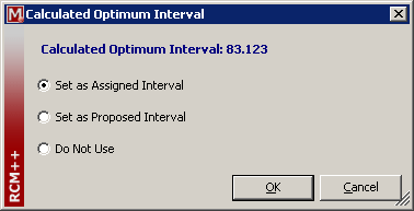
Figure 13: Specifying How the Calculated Optimum Interval Will Be Used

This optimum interval for preventive maintenance, 83.123 days, corresponds to the value obtained using BlockSim's Optimum Replacement tool, and both confirm the approximate value determined using the Optimum Replacement report template in Weibull++.