Comparing Two Products Using a Single Metric
[Editor's Note: This article has been updated since its original publication to reflect a more recent version of the software interface.]
A common task for a reliability engineer is to determine if one product is better than another. Often, comparison of a single metric, such as the time by which X% of the population is expected to fail (also known as the BX life), is used to answer the question of which product is superior. This article will illustrate two graphical methods to compare the B10 lives of two different designs using ReliaSoft's Weibull++ software.
Example
Joe has been assigned the task of determining whether a product that he buys from Vendor A can be replaced with a product from Vendor B. He knows that his budget will allow up to 10% returns during the warranty period, so Joe wants to compare the B10 lives of the products. He has the results of the original life test done previously on product A, and he has 5 samples of the new product, which he tests to failure. The results of these tests are shown in Table 1.
Table 1 -
Times-to-Failure of Products A and B in Hours
| Product A | Product B |
| 300 | 402 |
| 449 | 1116 |
| 587 | 1166 |
| 619 | 1233 |
| 700 | 1460 |
| 958 | |
| 2129 | |
| 2208 | |
| 2279 | |
| 2793 |
He enters the data into two Data Sheets in a Standard Folio and renames these sheets Product A and Product B. He knows from previous experience with this product that it will fail due to wear-out, so he computes the Weibull distribution parameters for each data set. The computed parameters are shown in Figures 1 and 2.
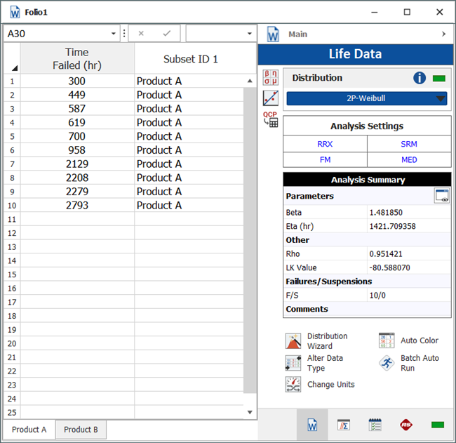
Figure 1: The Product A Data
Set
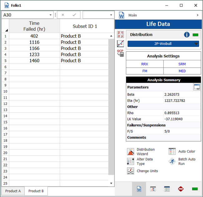
Figure 2: The Product B Data Set
Joe decides to compare the B10 lives of his two products by looking at the probability plots for each data set on the same graph. He right-clicks the Multiplots folder in the Project Explorer and chooses Add Overlay Plot. In the Select Data Sheets window, Joe chooses the data sets for both products, as shown in Figure 3, and then clicks OK.
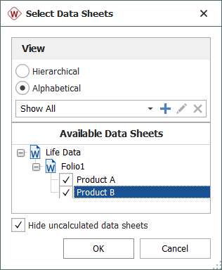
Figure 3: Selecting Data Sets
for the Multiplot
He knows that for a given unreliability (10%), he wants to see the variability in time (B10 life), so Joe chooses to add confidence bounds on time (also called "Type I" confidence bounds) to the plot. He shows these bounds on the plot by right-clicking within the plot and choosing Confidence Bounds from the shortcut menu that appears. He makes the selections shown in Figure 4 to put 90% two-sided bounds on the plot.
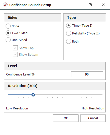
Figure 4: Setting Up Confidence
Bounds to Determine Variability in B10 Life
After Joe changes the line colors and styles for the confidence bounds using the Plot Setup, Joe's plot looks like the one shown in Figure 5.
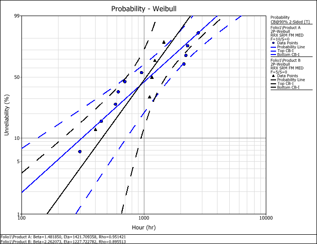
Figure 5: The Probability Plots
for Products A and B with Confidence Bounds.
Note that the blue curve and dotted lines represent product A, while the black curve and dashed lines represent Product B. Since the confidence bounds for Product A surround the Product B probability line and the confidence bounds for Product B surround the Product A probability line at a 10% unreliability, Joe concludes that there is no statistical difference between the B10 lives of the products from Vendors A and B. It is worth noting that this may not mean that the products from the two vendors actually have the same reliability/B10 life-- this is a small data set, and the wide confidence bounds indicate that there is simply not enough data to draw a firm conclusion.
Joe decides to prepare a report for his manager. He right-clicks the Reports folder in the Project Explorer and chooses Add ReliaSoft Workbook. In the Report Wizard, Joe leaves the Default Data Source field empty and verifies that the Based on an existing template check box is cleared, as shown in Figure 6.
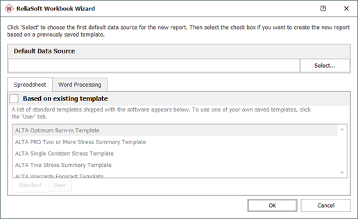
Figure 6: Setting up a Blank
Report
He then clicks OK. He types column headings and labels into the report as shown in Figure 7.
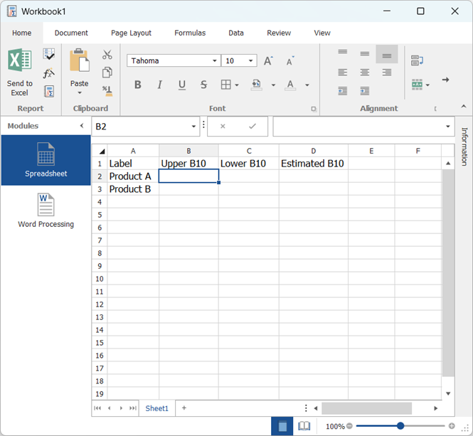
Figure 7: Creating Headings and
Labels for the Report
With cell B2 selected, Joe clicks the Function Wizard icon.

He chooses the TIMEATPF function and enters the information as shown in Figure 8 to calculate the upper bound on the B10 life at the 95% one-sided confidence level. (Note that this is equivalent to the 90% two-sided bound plotted in Figure 5.)
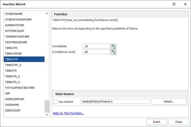
Figure 8: Using the Function
Wizard to Compute the Upper Bound on B10 Life for Product A
Joe clicks Insert to put the value of 719 hours into cell B2 in the report. In a similar manner, he uses the Function Wizard to obtain the complete table shown in Figure 9. (Note that the confidence level in the Function Wizard is 0.05 to calculate the values in the Lower B10 column and is left blank to calculate the values in the Estimated B10 column.)
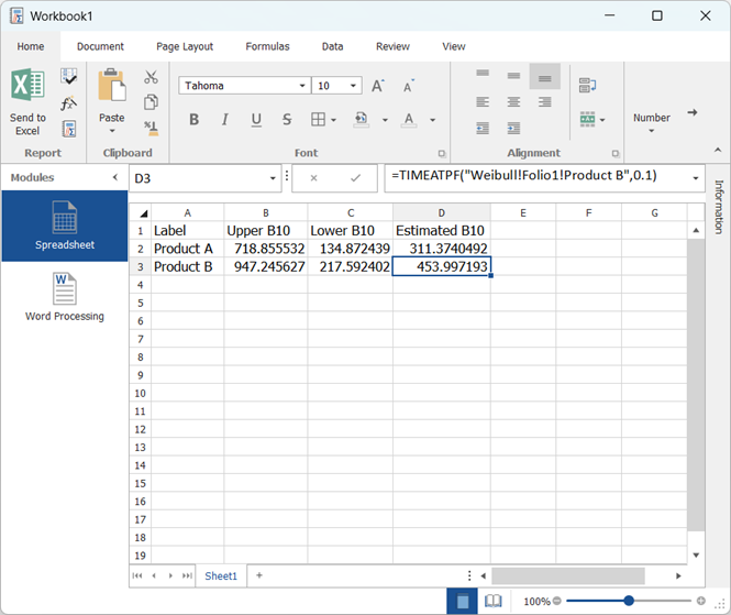
Figure 9: The Completed Table
of B10 Lives for Products A and B
Joe adds a graph to the report as follows. He highlights cells A1 through D3, and then clicks the Chart Wizard icon.

The cursor becomes a bold cross. He places the cursor at the top left of where he wants the chart to be located in the report, then clicks and drags the cursor to the bottom right of the desired location. When he releases the mouse button, the Chart Wizard appears. Joe does the following in the Chart Wizard:
- Gallery Page: chooses Hi Lo chart type
- Style Page: chooses chart style 3
- Layout Page: enters B10 Comparison as the chart title
- Axes Page: enters B10 Life (hours) as the Value (Y) axis title
Joe then clicks Finish to create the chart. Figure 10 shows the report.
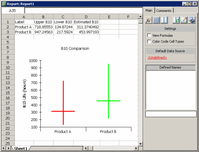
Figure 10: Graphical Display of
the Results in the Report
Since he can draw a horizontal line that intersects both data sets, he again concludes that he cannot tell a difference in the B10 lives of the products from Vendors A and B.
Conclusion
This article discussed two graphical methods to compare two data sets using the B10 life metric. Weibull++ also allows you to calculate the BX life for an individual data set using the Quick Calculation Pad (QCP). You may find this to be a quick and easy way to determine the B10 life in cases where you only need the metric. However, for times when you need to present the information graphically for maximum impact or rapid understanding, the methods presented in this article will be appropriate.