Analysis of Variance

[Editor's Note: This article has been updated since its original publication to reflect a more recent version of the software interface.]

Analysis of variance, or ANOVA, is a powerful statistical technique that involves partitioning the observed variance into different components to conduct various significance tests. This article discusses the application of ANOVA to a data set that contains one independent variable and explains how ANOVA can be used to examine whether a linear relationship exists between a dependent variable and an independent variable.

Sum of Squares and Mean Squares

The total variance of an observed data set can be estimated using the following relationship:

where:

• s is the standard deviation.
• yi is the ith observation.
• n is the number of observations.
• is the mean of the n observations.

The quantity in the numerator of the previous equation is called the sum of squares. It is the sum of the squares of the deviations of all the observations, yi, from their mean, . In the context of ANOVA, this quantity is called the total sum of squares (abbreviated SST) because it relates to the total variance of the observations. Thus:

The denominator in the relationship of the sample variance is the number of degrees of freedom associated with the sample variance. Therefore, the number of degrees of freedom associated with SST, dof(SST), is (n-1). The sample variance is also referred to as a mean square because it is obtained by dividing the sum of squares by the respective degrees of freedom. Therefore, the total mean square (abbreviated MST) is:

When you attempt to fit a model to the observations, you are trying to explain some of the variation of the observations using this model. For the case of simple linear regression, this model is a line. In other words, you would be trying to see if the relationship between the independent variable and the dependent variable is a straight line. If the model is such that the resulting line passes through all of the observations, then you would have a "perfect" model, as shown in Figure 1.

Figure 1: Perfect Model Passing Through All Observed Data Points

The model explains all of the variability of the observations. Therefore, in this case, the model sum of squares (abbreviated SSR) equals the total sum of squares:

For the perfect model, the model sum of squares, SSR, equals the total sum of squares, SST, because all estimated values obtained using the model, , will equal the corresponding observations, yi.

The model sum of squares, SSR, can be calculated using a relationship similar to the one used to obtain SST. For SSR, we simply replace the yi in the relationship of SST with :

The number of degrees of freedom associated with SSR, dof(SSR), is 1. (For details, click here.)

Therefore, the model mean square, MSR, is:

Figure 2 shows a case where the model is not a perfect model.

Figure 2: Most Models Do Not Fit All Data Points Perfectly

You can see that a number of observed data points do not follow the fitted line. This indicates that a part of the total variability of the observed data still remains unexplained. This portion of the total variability, or the total sum of squares that is not explained by the model, is called the residual sum of squares or the error sum of squares (abbreviated SSE). The deviation for this sum of squares is obtained at each observation in the form of the residuals, ei:

The error sum of squares can be obtained as the sum of squares of these deviations:

The number of degrees of freedom associated with SSE, dof(SSE), is (n-2). (For details, click here.)

Therefore the residual or error mean square, MSE, is:

Analysis of Variance Identity

The total variability of the observed data (i.e., the total sum of squares, SST) can be written using the portion of the variability explained by the model, SSR, and the portion unexplained by the model, SSE, as:

The above equation is referred to as the analysis of variance identity.

F Test

To test if a relationship exists between the dependent and independent variable, a statistic based on the F distribution is used. (For details, click here.) The statistic is a ratio of the model mean square and the residual mean square.

For simple linear regression, the statistic follows the F distribution with 1 degree of freedom in the numerator and (n-2) degrees of freedom in the denominator.

Example

Table 1 shows the observed yield data obtained at various temperature settings of a chemical process. We can analyze this data set using ANOVA to determine if a linear relationship exists between the independent variable, temperature, and the dependent variable, yield.

Table 1: Yield Data Observations of a Chemical Process at Different Values of Reaction Temperature

The parameters of the assumed linear model are obtained using least square estimation. (For details, click here.) These parameters are then used to obtain the estimated values, . The model sum of squares for this model can be obtained as follows:

The corresponding number of degrees of freedom for SSR for the present data set is 1.

The residual sum of squares can be obtained as follows:

The corresponding number of degrees of freedom for SSE for the present data set, having 25 observations, is n-2 = 25-2 = 23.

The F statistic can be obtained as follows:

The P value corresponding to this statistic, based on the F distribution with 1 degree of freedom in the numerator and 23 degrees of freedom in the denominator, is 4.17E-22. In this context, the P value is the probability that an equal amount of variation in the dependent variable would be observed in the case that the independent variable does not affect the dependent variable. (For more details about P values, click here.) Since this value is very small, we can conclude that a linear relationship exists between the dependent variable, yield, and the independent variable, temperature.

Weibull++

The above analysis can be easily carried out in ReliaSoft's Weibull++ software using the Multiple Linear Regression folio. Figure 3 shows the data from Table 1 entered into the folio and the results. You can see that the results shown in Figure 4 match the calculations shown previously and indicate that a linear relationship does exist between yield and temperature.

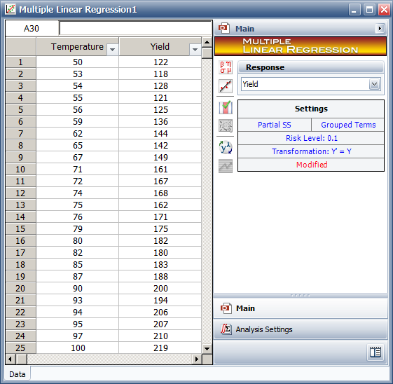
Figure 3: Data Entry in Weibull++ for the Observations in Table 1

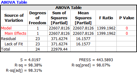
Figure 4: ANOVA Table for the Data in Table 1

References

[1] ReliaSoft Corporation, Experiment Design and Analysis Reference, Tucson, AZ: ReliaSoft Publishing, 2008.
[2] Montgomery, D., Design and Analysis of Experiments, 5th edition, 2001, New York: John Wiley & Sons, 2001.
[3] Kutner, Michael H., Nachtsheim, Christopher J., Neter, John, and Li, William, Applied Linear Statistical Models, New York: McGraw-Hill/Irwin, 2005.