Reliability Requirements and Specifications

One of the most essential aspects of a reliability program is defining the reliability goals that a product needs to achieve. This article will explain the proper ways to describe a reliability goal and also highlight some of the ways reliability requirements are commonly defined improperly.

Designs are usually based on specifications. Reliability requirements are typically part of a technical specifications document. They can be requirements that a company sets for its product and its own engineers or what it reports as its reliability to its customers. They can also be requirements set for suppliers or subcontractors. However, reliability can be difficult to specify. It is easy to use "qualitative" language such as, "our product needs to exceed customer expectations" or "our product should be more reliable than its competition." Joseph Juran, a famous quality pioneer, said, "If you don't measure it, you don't manage it." If an organization does not specify reliability goals numerically, it loses control over managing its products' reliability improvements.

What are the essential elements of a reliability requirement?

There are many facets to a reliability requirement statement.

Measurable:
Reliability metrics are best stated as probability statements that are measurable by test or analysis during the product development time frame.

Customer usage and operating environment:
The demonstrated reliability goal has to take into account the customer usage and operating environment. The combined customer usage and operating environment conditions must be adequately defined in product requirements. Many types of stresses or customer behaviors can be combined to describe the usage and operating environment. The descriptions can be done in many ways. For instance:

• Using constant values. For example: Usage temperature is 25°C. This could be an average value or, preferably, a high stress value that accommodates most customers and applications.

• Using limits. For example: Usage temperature is between -15°C and 40°C.

• Using distributions. For example: Usage temperature follows a normal distribution with mean of 35° C and standard deviation of 5°C.

• Using time-dependent profiles. For example: Usage temperature starts at 70°C at t = 0, increases linearly to 35°C within 3 hours, remains at that level for 10 hours, then increases exponentially to 50°C within 2 hours and remains at that level for 20 hours. A mathematical model (function) can be used to describe such profiles.

Time:
Time could mean hours, years, cycles, mileage, shots, actuations, trips, etc. It is whatever is associated with the aging of the product. For example, saying that the reliability should be 90% would be incomplete without specifying the time window. The correct way would be to say that, for example, the reliability should be 90% at 10,000 cycles.

Failure definition:
The requirements should include a clear definition of product failure. The failure can be a complete failure or degradation of the product. For example: part completely breaks, part cracks, crack length exceeds 10 mm, part starts shaking, etc. The definition is incorporated into tests and should be used consistently throughout the analysis.

Confidence:
A reliability requirement statement should be specified with a confidence level, which allows for consideration of the variability of data being compared to the specification.

Understanding Reliability Requirements

Assuming that customer usage and operating environment conditions and what is meant by a product "failure" have already been defined, let us examine the probability and life element of a reliability specification. We will look at some common examples of reliability requirements and understand what they mean. We will use an automotive product for illustration.

Requirement Example 1:  Mean  Life (MTTF) = 10,000 miles

The Mean Life (or Mean-Time-To-Failure [MTTF]) as a sole metric is flawed and misleading. It is the expected value of the random variable (mean of the probability distribution). Historically, the use of MTTF for reliability dates back to the time of wide use of the exponential distribution in the early days of quantitative reliability analysis. The exponential distribution was used because of its mathematical (computational) simplicity. The exponential distribution has just one parameter, the MTTF (or its reciprocal, the "failure rate," which is constant, thus the reason for its simplicity). Few products and components actually have a constant failure rate (i.e., no wearout, degradation, fatigue, infant mortality, etc.).

The MTTF might be one of the most misunderstood metrics among reliability engineering professionals. Some interpret it as "no failure by 10,000 miles," which is wrong! Some interpret it as "by 10,000 miles, 50% of the product's population (50th percentile) will fail." The "mean," however, is not the same as the "median," so this is only true in cases where the product failure distribution is a symmetrical distribution, such as the normal distribution. If the product follows a non-symmetrical distribution (such as Weibull, lognormal and exponential), which is usually the case in reliability analysis situations, then the mean does not necessarily describe the 50th percentile, but could be the 20th percentile, 70th, 90th, etc., depending on the distribution type and the estimated parameters of that distribution. In the case of the exponential distribution, the percentile that matches the mean life is actually the 63.2%! If the intention of using the mean life as a metric is to describe the time by which 50% of the product's population will fail, then the appropriate metric to use would be the B50 life.

Let us use the following example for illustration. A company tested 8 units of a product manufactured by two different suppliers. The failure results are shown next.

The two different data sets were modeled using a Weibull distribution and rank regression based on X (RRX). The MTTFs calculated based on the two different distributions are:

• MTTF₁ = 9999.6 miles

• MTTF₂  = 9999.4 miles

 

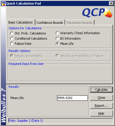
These MTTFs are almost the same. So, based on this type of reliability metric, the two suppliers' reliability can be considered to be equal.

Now, let us look at the reliability plots for the two suppliers' failure distributions.

After examining the above plot, does the conclusion that the two suppliers' reliability is almost the same still hold true? Even though the two suppliers' MTTFs are almost the same, the above plot indicates that their reliabilities are significantly different. For example, Supplier 1's reliability at 10,000 miles is 36.79%, whereas Supplier 2's reliability at 10,000 miles is 50.92%. This is a considerable difference in reliability.

In this example, because the Weibull distribution is not a symmetrical distribution, the MTTFs do not correspond to the 50th percentile of failures. The actual percentiles can be calculated using the reliability function. The percentile, P, of units that would fail by t = MTTF is:

• P₁ = Q(MTTF₁) = 1-R(t = MTTF₁) = 63.21%

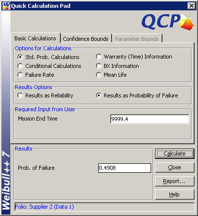
• P₂ = Q(MTTF₂) = 1-R(t = MTTF₂) = 49.08%

The 50th percentile of failures can be computed using the B50 metric.

• B50₁ = 6,930 miles

• B50₂ = 10,066 miles

Attempting to use a single number to describe an entire lifetime distribution can be misleading and may lead to poor business decisions.

Requirement Example 2:  MTBF = 10,000 miles.

Unfortunately, the term MTBF (Mean-Time-Between-Failures) has often been used in place of MTTF (Mean-Time-To-Failures). Many reliability textbooks and standards erroneously intermix these terms. MTTF and MTBF are the same only in the case of a constant failure rate (exponential distribution assumption). MTBF should be used when dealing with repairable systems, whereas MTTF should be used when looking for the mean of the first time-to-failure (i.e., non-repairable systems).

Requirement Example 3:  Failure rate = 0.0001 failures per mile.

The use of failure rate as a reliability requirement implies an exponential distribution, since this is the only distribution commonly used for reliability (life data) analysis that has a constant failure rate. For the exponential distribution, MTTF = 1/Failure Rate = 1/0.0001 = 10,000 miles. Thus, this reliability requirement is equivalent to Example 1. Most distributions used for life data analysis have a failure rate that varies with time. In these cases, MTTF is not equal to 1/Failure Rate. Consequently, the only way that using a failure rate for a reliability requirement would make sense for distributions other than the exponential distribution would be if a time were also specified.

Requirement Example 4: B10 life = 10,000 miles.

BX refers to the time by which X% of the units in a population will have failed. This metric has its roots in the ball and roller bearing industry. It then found its way to other industries and is now just a statistical metric that is widely used. This reliability requirement means that 10% of the population will fail by 10,000 miles. Or, in other words, the reliability of the product is 90% at 10,000 miles. This metric is a good metric because it does not make the exponential distribution assumption and also because it states clearly the percentile of failures by a certain time value.

Requirement Example 5: 90% Reliability at 10,000 miles.

This is equivalent to the previous example.

• The time of interest is 10,000 miles. This could be design life, warranty period or whatever operation/usage time is of interest to you and your customers.

• The probability that the product will not fail before 10,000 miles is 90%. Or, there is a probability that 10% will fail by 10,000 miles.

Although the above two examples (4 and 5) are good metrics, they lack a specification of how much confidence is to be had in estimating whether the product meets these reliability goals.

Requirement Example 6: 90% Reliability at 10,000 miles with 50% confidence.

Same as above (Example 5) with the following addition:

• The lower reliability estimate obtained from your tested sample (or data collected from the field) is at the 50% confidence level.

This corresponds to the regression line that goes through the data in a regression plot obtained when a distribution (such as a Weibull) model is fitted to times-to-failure. The line is at 50% confidence. In other words, this means that there is a 50% chance that your estimated value of reliability is greater than the true reliability value and there is a 50% chance that it is lower. Using a lower 50% confidence on reliability is equivalent to not mentioning the confidence level at all!

Let us use the following example to illustrate calculating this reliability requirement.

The two designs are modeled with a Weibull distribution and using rank regression on X as the parameter estimation method. The following figure shows the probability plot for the two designs.

The above plot shows that at 10,000 miles, the demonstrated reliability of Design B (96.81%) is superior to Design A's demonstrated reliability (95.93%) at the 50% confidence (along the probability line). Both designs meet the reliability requirement; however, the demonstrated reliability of B is better.

Requirement Example 7: 90% Reliability for 10,000 miles with 90% confidence.

Same as above (Example 6) with the exception that here, more confidence is required in the reliability estimate. This statement means that the 90% lower confidence estimate on reliability at 10,000 miles should be 90%.

If we show the above probability plot with the 90% one-sided confidence bounds, obtained using the Fisher matrix confidence bounds method, we get the following:

The above plot shows that at 10,000 miles, the 90% lower bound on reliability is 79.27% for Design B and 90.41% for Design A. Unlike in the previous example, here, the demonstrated reliability of A is better than that of B and only A is demonstrated to meet the reliability requirement. The way this reliability requirement is stated is better then the requirement of the previous example. In this example, the requirement is able to uncover the sample size issue and its effect on reliability analysis.

Requirement Example 8: 90% Reliability for 10,000 miles with 90% confidence for a 98th percentile customer.

Same as above (Example 7) with the following addition:

• The 98th percentile is a point on the usage stress curve. This describes the stress severity level for which the reliability is estimated. It means that 98% of the customers who use the product, or 98% of the range of environmental conditions applied to the product, will experience the 90% reliability.

To be able to estimate reliability at the 98th percentile of the stress level, units would have to be tested at that stress level or, using accelerated testing methods, the units could be tested at different stress levels and the reliability could be projected to the 98th percentile of the stress.

Conclusion

As demonstrated in this article, it is important to understand what a reliability requirement actually means in terms of product performance and to select the metric that will accurately reflect the expectations of the designers and end-users. The MTTF, MTBF and failure rate metrics are commonly misunderstood and very often improperly applied. Whereas, the BX life or the reliability at a given time are more appropriate metrics because they can be calculated for any of the statistical distributions commonly used to analyze product lifetime data and they describe specific, measurable expectations. Such metrics can be improved by specifying a confidence level to account for variability within the data and by clearly defining the anticipated user-stress level for which the estimates are made. Therefore, demonstrating that a product meets a reliability specification such as "90% Reliability for 10,000 miles with 90% confidence for a 98th percentile user" provides the greatest likelihood that actual performance will match the estimates.