Availability and the Different Ways to Calculate It
[Editor's Note: This article has been updated since its original publication to reflect a more recent version of the software interface.]
Availability is an important metric used to assess the performance of repairable systems, accounting for both the reliability and maintainability properties of a component or system. Did you know, though, that there are different classifications of availability and different ways to calculate it? This article will explore the different availability classifications, what they mean and how they can be calculated with the help of BlockSim.
Availability Classifications
The classification of availability is somewhat flexible and is largely based on the types of downtimes used in the computation and on the relationship with time (i.e., the span of time to which the availability refers). As a result, there are a number of different classifications of availability, including:
-
Instantaneous (or Point) Availability
-
Average Uptime Availability (or Mean Availability)
-
Steady State Availability
-
Inherent Availability
-
Achieved Availability
-
Operational Availability
A wide range of availability classifications and definitions exist. The ones presented here are the most common but variations exist and you should be aware of how they are calculated and what they mean so that you can make an appropriate choice for the analysis you are performing.
Instantaneous or Point Availability, A(t)
Instantaneous (or point) availability is the probability that a system (or component) will be operational (up and running) at a specific time, t. This classification is typically used in the military, as it is sometimes necessary to estimate the availability of a system at a specific time of interest (e.g., when a certain mission is to happen). The point availability is very similar to the reliability function in that it gives a probability that a system will function at the given time, t. Unlike reliability, however, the instantaneous availability measure incorporates maintainability information. At a given time, t, the system will be operational if one of the following conditions is met (1):
-
The system functioned properly from 0 to t, i.e., it never failed by time t. The probability of this happening is R(t).
Or,
-
The system functioned properly since the last repair at time u, 0 < u < t. The probability of this condition is:
with m(u) being the renewal density function of the system.
Consequently, the point availability is the summation of the above two probabilities, or:
In BlockSim, the point availability can be obtained through simulation. It can be estimated for different points of time and can also be plotted as a function of time.
Average
Uptime Availability (or Mean Availability),

The mean availability is the proportion of time during a mission or time period that the system is available for use. It represents the mean value of the instantaneous availability function over the period (0, T] and is given by:
For systems that have periodical maintenance, availability may be zero at regular periodical intervals. In this case, mean availability is a more meaningful measure than instantaneous availability. Such a definition of availability is commonly used in manufacturing and telecommunication systems.
Steady
State Availability,

The steady state availability of the system is the limit of the availability function as time tends to infinity. Steady state availability is also called the long-run or asymptotic availability. A common equation for the steady state availability found in literature is:
However, it must be noted that the steady state also applies to mean availability.
The next figure illustrates the steady state availability graphically.
Figure 1
- Illustration of point availability approaching steady
state
For practical considerations, the availability function will start approaching the steady state availability value after a time period of approximately four times the average time-to-failure. This varies depending on the maintainability issues and complexity of the system. In other words, you can think of the steady state availability as a stabilizing point where the system's availability is roughly a constant value.
The steady state availability reflects the long-term availability after the system "settles." The system availability may initially be unstable due to training/learning issues, deciding on a good spare parts stocking policy, deciding on the number of repair personnel, optimizing the efficiency of repair, burn-in of the system, etc., and could take some time before it stabilizes.
It is important to be very careful in using the steady state availability as the sole metric for some systems, especially systems that do not need regular maintenance. A large-scale system with repeated repairs, such as a car, will reach a point where it is almost certain that something will break and need repair once a month. However, this state may not be reached until, for instance, 500,000 miles. Obviously, if an Operations Manager of rental vehicles, for example, keeps the vehicles until they reach 50,000 miles, then this metric value would not be of any use.
Inherent Availability, AI
Inherent availability is the steady state availability when considering only the corrective maintenance (CM) downtime of the system. This classification is what is sometimes referred to as the availability as seen by maintenance personnel. This classification excludes preventive maintenance downtime, logistic delays, supply delays and administrative delays. Since these other causes of delay can be minimized or eliminated, an availability value that considers only the corrective downtime is the inherent or intrinsic property of the system. Many times, this is the type of availability that companies use to report the availability of their products (e.g., computer servers) because they see downtime other than actual repair time as out of their control and too unpredictable.
The corrective downtime reflects the efficiency and speed of the maintenance personnel, as well as their expertise and training level. It also reflects characteristics that should be of importance to the engineers who design the system, such as the complexity of necessary repairs, ergonomics factors and whether ease of repair (maintainability) was adequately considered in the design.
For a single component, the inherent availability can be computed by:
This gets slightly more complicated for a system. To do this, you need to look at the mean time between failures, or MTBF, and compute this as follows:
|
MTBF = Uptime / Number of System Failures MTTR = CM Downtime / Number of System Failures |
This may look simple. However, you should keep in mind that until steady state is reached, the MTBF calculation may be a function of time (e.g., a degrading system). In such cases, before reaching steady state, the calculated MTBF changes as the system ages and more data are collected. Thus, the above formulation should be used cautiously. Furthermore, it is important to note that the MTBF defined here is different from the MTTF (or, more precisely for a repairable system, MTTFF: mean time to first failure).
Achieved Availability, AA
Achieved availability is very similar to inherent availability with the exception that preventive maintenance (PM) downtimes are also included. Specifically, it is the steady state availability when considering corrective and preventive downtime of the system. The achieved availability is sometimes referred to as the availability seen by the maintenance department (includes both corrective and preventive maintenance but does not include logistic delays, supply delays or administrative delays).
Achieved availability can be
computed by looking at the mean time between maintenance
actions, MTBM, and the mean maintenance downtime,  :
:
|
MTBM = Uptime / (Number of System Failures + Number of System Downing PMs)
|
Note: System Downing PMs are PMs that cause the system to go down or require a shut down of the system.
Operational Availability, Ao
Operational availability is a measure of the "real" average availability over a period of time and includes all experienced sources of downtime, such as administrative downtime, logistic downtime, etc. The operational availability is the availability that the customer actually experiences. It is essentially the a posteriori availability based on actual events that happened to the system. The previously discussed availability classifications are a priori estimates based on models of the system failure and downtime distributions. In many cases, operational availability cannot be controlled by the manufacturer due to variation in location, resources and other factors that are the sole province of the end user of the product.
Operational availability is the ratio of the system uptime to total time. Mathematically, it is given by:
where the operating cycle is the overall time period of operation being investigated and uptime is the total time the system was functioning during the operating cycle. (Note: The operational availability is a function of time, t, or operating cycle.)
The concept of operational availability is closely related to the concept of operational readiness. In military applications, this means that the assigned numbers of operating and maintenance personnel, the supply chain for spare parts and training are adequate. In the commercial world, a manufacturer may be capable of manufacturing a very reliable and maintainable product (i.e., very good inherent availability). But what if the manufacturer has a poor distribution and transportation system or does not stock the parts needed or provide enough service personnel to support the systems in the field? Then, the readiness of this manufacturer to go to market with the product is low.
Logistic planners, design engineers and maintainability engineers can collaboratively estimate the repair needs of the system, required personnel, spares, maintenance tasks, repair procedures, support equipment and other resources. Only when all downtime causes are addressed will you be able to paint a realistic picture of your system's availability in actual operation.
What Type of Availability Should You Use?
You may be wondering why there are so many types of availability and which one you should use. You can use different classifications of availabilities to present different conclusions about your system's availability. The difference can be potentially large and availability measurements can be misused or misleading to your company and your customers. If you use a different classification from the one your customer uses, you and your customer could have very different impressions of the system. Therefore, the choice of availability classification to use should be made carefully, taking into account your system and industry and how your company and your customers perceive availability. Another place to be careful about availability definition is in contracts. Definitions need to be stated clearly. Make sure that your company and your customers have the same understanding of availability and agree on the classification to use.
As an example, if your system has an increasing availability (as in the second part of Figure 1) and you report the long-term steady state availability of your system, but your customer judges your system based on the short-term mean availability, then you will have a problem. As another example, consider a company that rents oil drilling equipment and is responsible for repairing the equipment. If their customer penalizes them because the equipment stays down longer than a certain duration, they might consider using operational and mean availability metrics (that include all delays) in their analyses instead of inherent (or achieved) availability, which considers only the corrective (and preventive) actions downtime when parts and crews are available.
BlockSim Example
Let us use the following repairable system reliability block diagram to illustrate the different availability classifications and calculations using BlockSim.
The blocks have the following failure and repair properties.
| Component | Failure Distribution (hours) | Repair Duration Distribution (hours) | Preventive Replacement Policy | Preventive Replacement Duration Distribution (hours) | Repair and Preventive Parts Pool | Maintenance Crew Delay (Travel Time) (hours) |
| A | Weibull (β = 1.5, η = 1,000) |
Normal (μ =12, σ= 2) |
Every 1,000 hours based on system age | Normal (μ =5, σ= 1.5) |
Spare Part Pool A | Normal (μ =5, σ= 2.5) |
| B | Lognormal (μT' =5, σT'= 1) |
Exponential (Mean = 20) |
-- | -- | Spare Part Pool B | Normal (μ =5, σ= 2.5) |
| C |
Exponential (Mean = 10,000) |
Normal (μ =15, σ= 5) |
Every 1,000 hours based on system age | Normal (μ =5, σ= 1.5) |
Spare Part Pool C | Normal (μ =5, σ= 2.5) |
| D | Weibull (β= 3, η = 2,000) |
Exponential (Mean = 14) |
Every 1,000 hours based on system age | Normal (μ =5, σ= 1.5) |
Spare Part Pool D | Normal (μ =5, σ= 2.5) |
All the components share the same maintenance crew. The crew can perform only one task at a time.
The spare part pools have the following properties.
| Spare Part Pool | Initial Stock Level | Logistic Delay to Obtain Part from Pool | Pool Restocking | Logistic Delay (Shipping) to Restock Pool |
| Spare Part Pool A | 5 | Normal (μ =1,σ= 0.5) | Add 1 when stock drops to 1 | Normal (μ =96,σ= 3) |
| Spare Part Pool B | 20 | Normal (μ =1,σ= 0.5) | Add 1 when stock drops to 1 | Normal (μ =96,σ= 3) |
| Spare Part Pool C | 1 | Normal (μ =1,σ= 0.5) | Add 1 when stock drops to 0 | Normal (μ =96,σ= 3) |
| Spare Part Pool D | 2 | Normal (μ =1,σ= 0.5) | Add 1 when stock drops to 1 | Normal (μ =96,σ= 3) |
In this example, we are interested in the operation of the system over 3,000 hours.
The RBD is created and the failure and maintenance properties are set.
Calculating Instantaneous (or Point) Availability
Using the RBD model and all the repair characteristics and delays, the system is simulated for 3,000 hours of operation. The following figure for the instantaneous availability is then obtained.
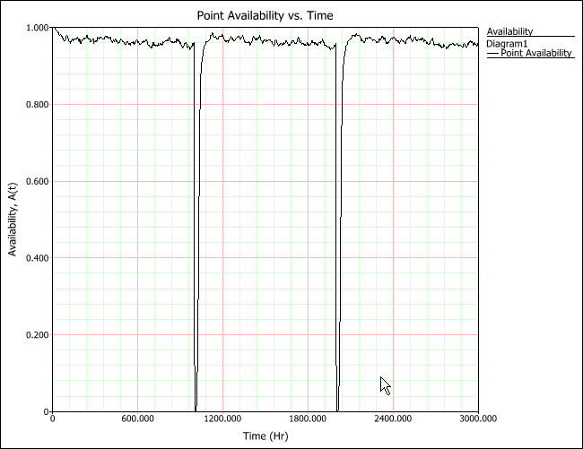
Figure 2: Instantaneous (or point) availability plot
As you can see in the above figure, the availability drops during the PMs. As an example of instantaneous availability calculations, the instantaneous availability at t = 500 is 0.9627, at t = 1,000 is 0.6400 and at t = 2,500 is 0.9703. The results can be read directly from the graph or obtained using the Quick Calculation Pad (QCP).
Calculating Average Uptime Availability (or Mean Availability)
Using the RBD model and all the repair characteristics and delays, the system is simulated for 3,000 hours of operation. The mean availability can be obtained using the Quick Calculation Pad (QCP), as shown next, or by reading the value from the summarized simulation report.
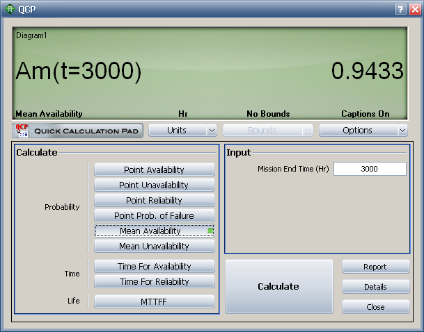
In this example, the mean availability at 3,000 hours is 0.9433.
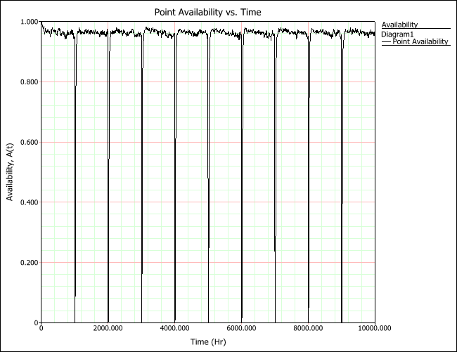
Calculating Steady State Availability
To obtain the long-term availability of the system, we simulate it for a much longer time, 10,000 hours. In this example, there is actually no obvious steady state in terms of the point availability. The system is renewed by the PMs and the availability increases again, as can be seen in the following instantaneous (or point) availability plot. In addition, the PMs are performed based on predetermined system age intervals, where the system "goes down" during the PM, causing point availability to be zero during these intervals.
Calculating Inherent Availability
To calculate the inherent availability, AI, for this example, we need to simulate the system with corrective maintenance downtime without logistic delays or preventive maintenance. All of these characteristics should be disabled in the BlockSim model in order to obtain the intrinsic availability of the system. To calculate AI, we need to calculate the MTBF and MTTR.
|
MTBF (Uptime) |
= Uptime / Number of System Failures |
|
= 2,892.9236/6.248 |
|
|
= 463.0159 hours |
|
|
MTTR |
= CM Downtime / Number of System Failures |
|
|
= 107.0764 / 6.248 |
|
= 17.1377 hours |
The values of uptime, number of system failures and CM downtime are all obtained from the System Overview report in BlockSim, as shown next.
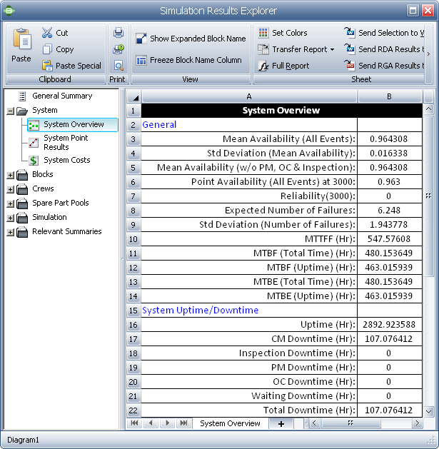
Therefore:
AI = MTBF / (MTBF + MTTR) = 0.9643
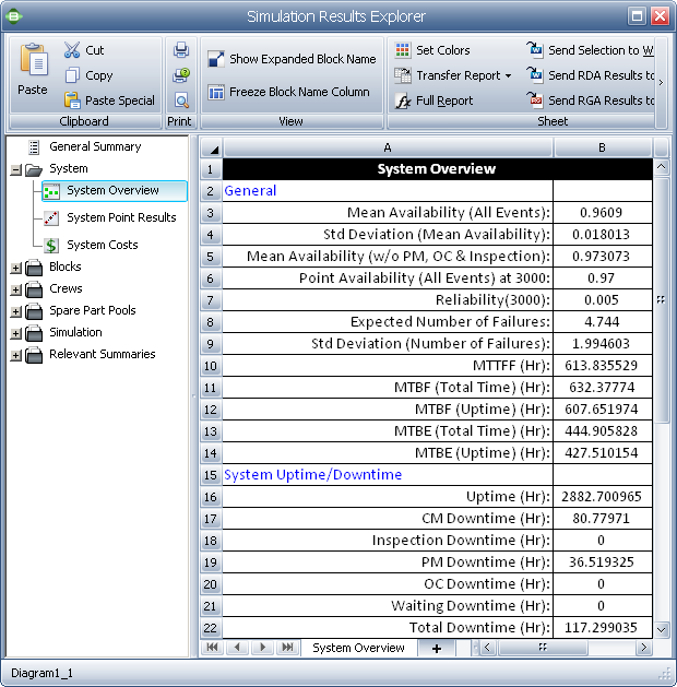
Calculating Achieved Availability
To calculate the achieved
availability for this example, we need to simulate the
system with corrective and preventive maintenance downtimes
but without logistic delays (all logistic delay
characteristics should be disabled in the BlockSim
model). The estimated achieved availability is obtained by
calculating MTBM and
![]() .
.
|
MTBM |
= Uptime / (Number of System Failures + Number of System Downing PMs) |
|
= 2882.7010 / 6.743 |
|
|
= 427.5102 |
|
|
|
= (CM Downtime + PM Downtime) / (Number of System Failures + Number of System Downing PMs) |
|
= 117.2990 / 6.743 |
|
|
= 17.3957 |
The values of uptime, number of system failures, CM Downtime, PM Downtime, number of system failures and number of system downing PMs are all obtained from the System Overview report in BlockSim, as shown next.
Therefore:
AA
= MTBM / (MTBM +![]() )
= 0.9609
)
= 0.9609
Calculating Operational Availability
This is calculated in
BlockSim similarly to the mean availability
calculation. The operational availability is expected to be
0.9433.
Note: This estimate is based on the model, not on actual
observation of operation. There are other factors (not
included in this model) that could affect the operational
availability, such as customer delays, additional travel
time, etc.Typically, operational availability is
calculated based on actual observed events, not on the
model. This model can serve only as an a priori
estimate of the operational availability and can be fine
tuned by adding more expected delays that a customer can
observe.
Conclusion
This article discussed the different classifications and ways to calculate the availability of repairable systems. This type of availability for your application should be considered carefully because different classifications can give very different results about the system's availability. The article also demonstrated how BlockSim can be used to make these different calculations.
References
1- Elsayed, E., Reliability Engineering, Addison Wesley, Reading, MA, 1996.