Time Varying and Multi-Phase Throughput Analysis

Reliability Block Diagram (RBD) models are generally used to describe the reliability-wise configuration of a system but they can also be used to represent the system's production/processing sequence. In such cases, we can take system analysis through RBDs a step further and utilize them to study the productivity or yield of the system via throughput analysis. This is applicable when the system can process (or make) something, such as manufacturing systems, chemical processes and oil refineries. Throughput analysis has been discussed before in this e-magazine; in this article we discuss the modeling and analysis of phased and time varying throughput with the help of BlockSim 7.

This article combines concepts of throughput analysis and Reliability Phase Diagrams (RPDs). For more information about throughput analysis, click here. To find out more about RPDs, click here. You can also read an article about RPD analysis in the latest issue of the Reliability Edge.

Applications for This Type of Analysis

Time varying and multi-phase throughput can be found in many industry applications. For example, consider a textile factory that receives different quantities of raw materials during different seasons. These seasons could be treated as different phases.

Another example is the start up period in a processing plant. When the plant stops operating, due to planned or unplanned maintenance, the equipment requires a warm up period before reaching its maximum production capacity. The methodology used for variable throughput is discussed next.

Variable (Time Varying) Throughput

In BlockSim 7, time varying throughput can be specified at the phase level through the Variable Throughput property of an operational phase. Variable throughput permits modeling of scenarios where the throughput changes over time. Three general models for variable throughput are available in BlockSim. Each of these models has two parameters, which are specified by the user. These models are discussed below:

1) Linear model: y = ax + b

This model describes the change in throughput y as a linear function of time x. The total throughput processed between any two points of time x1 and x2 is obtained by integration of the linear function as:

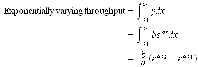
2) Exponential model: y = beax

This model describes the change in throughput y as an exponential function of time x. The total throughput processed in a period of time between any two points x1 and x2 is obtained as:

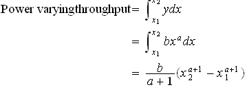
3) Power model: y = bxa

This model describes the change in throughput y as a power function of time x. The total throughput processed between two points of time x1 and x2 is obtained as:

All of the above models also have a user-defined maximum throughput capacity value. If this maximum throughput capacity value is reached, the throughput per unit time becomes constant at that value. In this situation, the variable throughput model then acts as a constant throughput model. The above models may at first glance seem limited, but they do in fact provide ample modeling flexibility. This flexibility is achieved by using these functions as building blocks for more complex functions. For example, a step model can be easily created by using multiple phases, each with a constant throughput. A ramp model would use phases with linearly increasing functions in conjunction with constant phases, and so forth. In addition, decreasing throughput can be modeled by manipulation of the parameters.

Example

We will use a simple example to illustrate the use of BlockSim 7 to model phase and time varying throughput.

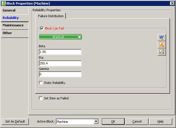
A production machine follows a Weibull distribution with β = 1.55 and η = 250.4 days. When an outage happens, it takes about 12 days to restore the machine.

The above figure represents the Reliability Block Diagram (RBD) of the machine. The failure properties are shown next.

Every time the machine fails, the machine is repaired then the throughput of the machine goes through a warm up period of 5 days until it reaches normal production capacity again. The throughput in units per day can be described as follows:
 

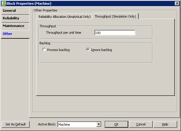
The normal operation throughput is specified in the machine's properties window, as shown next (no backlog is specified for this example).

To model the two-phase operation (warm up and normal operation) of this machine, a Reliability Phase Diagram (RPD) is used, as shown next.

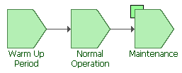
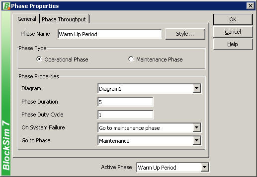
Both the Warm Up Period and Normal Operation phases in the above RPD are linked to the same Diagram Sheet, which contains the machine's RBD. The following figures show the phase properties of these first two phases. In addition to the linked diagram, the phase properties also specify the duration of the phase and what action is to be taken if a system failure occurs. In this case, the action upon system failure is to go to a maintenance phase, which is specified in the next field. Once the maintenance phase has been executed, the system will then go through warm up again.

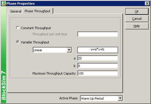
The warm up phase has a variable throughput, specified as follows.

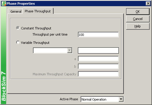
The normal operation phase has a constant throughput, as shown next.

The maintenance phase is defined in BlockSim 7 as a template that contains the blocks to be fixed in the RBD and their associated repair properties (such as repair times, resources, etc.) Note that while repairs may be performed during an operational phase, a maintenance phase is exclusively dedicated to the execution of maintenance tasks.

The repair properties for the block in the maintenance template are shown next.

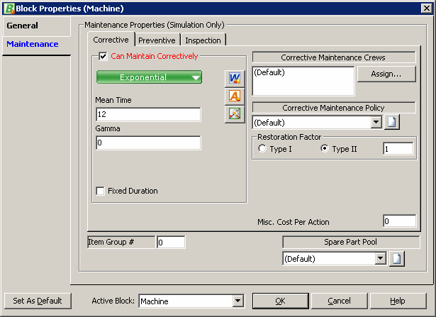
The system is simulated for 1092 days (3 years) with 156 increments for weekly results. On the Throughput Settings tab of the Maintainability/Availability Simulation window, Report Throughput Point Results is selected, as shown next.

A System Overview summary of the simulation is shown next (note that your results may vary slightly since they were obtained via simulation).

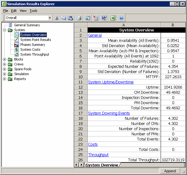
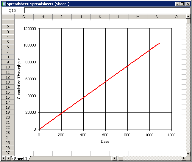
The mean availability of the system for the next three years is estimated to be 95.41% and the expected throughput of the plant at the end of three years is expected to be 102,719.31 units. 

For an overview of the plants availability as a function of time, you can generate a point availability plot like the one shown next. 

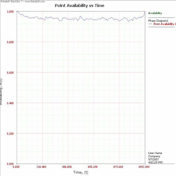
The point results of the throughput as a function of time can also be obtained from the System Point Results report. The following is a plot of the cumulative throughput over time.

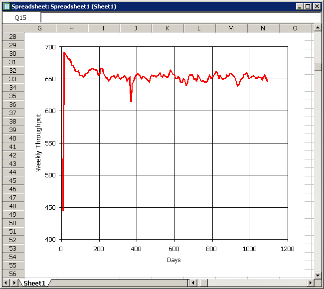
The following is a plot of the weekly throughput.