On-Condition Maintenance Using P-F Interval or Failure Detection Threshold (FDT)

[Editor's Note: This article has been updated since its original publication to reflect a more recent version of the software interface.]

On-condition maintenance relies on the capability to detect failures before they happen so that preventive maintenance can be initiated. Many failure modes exhibit signs of warning as they are about to occur. If, during an inspection, maintenance personnel can find evidence that the equipment is approaching the end of its life, then it may be possible to delay the failure, prevent it from happening or replace the equipment at the earliest convenience rather then allowing the failure to occur and possibly cause severe consequences. This article explains a methodology, using Weibull++, to estimate the P-F interval or Failure Detection Threshold (FDT), which are two typical ways to describe the detectability of a failure. In addition, this article shows how to use the detectability information on condition tasks for use in the analysis of repairable systems in BlockSim or RCM++.

Background

In the arena of Reliability Centered Maintenance (RCM) or repairable system analysis, one of the strategies for failure management is on-condition maintenance, also called predictive or condition-based maintenance. This strategy relies on the capability of maintenance personnel to detect potential failures in advance in order to take appropriate actions. Examples of failure signs that can be detected are vibrations, cracks, particles in oil, temperature, noise, viscosity, color, etc. Many technologies have been developed to monitor failure characteristics such as vibration analysis, X-ray radiography, ultrasonics, infrared thermography, oil analysis, acoustic emission, etc.

P-F Curves and P-F Intervals

A common curve that illustrates the behavior of equipment as it approaches failure is the P-F curve. The curve shows that as a failure starts manifesting, the equipment deteriorates to the point at which it can possibly be detected (P). If the failure is not detected and mitigated, it continues until a "hard" failure occurs (F). The time range between P and F, commonly called the P-F interval, is the window of opportunity during which an inspection can possibly detect the imminent failure and address it. P-F intervals can be measured in any unit associated with the exposure to the stress (running time, cycles, miles, etc). For example, if the P-F Interval is 200 days and the item will fail at 1,000 days, the approaching failure begins to be detectable at 800 days.

Failure Detection Threshold (FDT)

In addition to P-F intervals, the indication of when the approaching failure will become detectable during inspections can be specified using a factor called the Failure Detection Threshold (FDT). FDT is a number between 0 and 1 that indicates the percentage of an items life that must elapse before an approaching failure can be detected. For example, if the FDT is 0.9 and the item will fail at 1,000 days, the approaching failure becomes detectable after 90% of the life has elapsed, which translates to 900 days in this case (0.9 * 1,000 = 900).

Estimating the P-F Interval or FDT

Estimation of the P-F interval or FDT can be achieved using the judgment and experience of the people who design, manufacture and/or operate the equipment. Note that estimating the P-F Interval or FDT should be done on one failure mode at a time.

Many failure mechanisms can be directly linked to the degradation of part of the product. Weibull++'s degradation analysis folio enables the analysis of degradation data. Degradation analysis involves the measurement of the degradation of performance/quality data that can be directly related to the presumed failure of the product in question. Assuming such data can be obtained, the FDT or P-F Interval can be estimated using this technique.

To illustrate the use of this method, we use an example from an oil refinery company that performed a study on the clogging problem in a type of pipes in its refinery. A type of inspection equipment that uses gamma rays to measure the thickness of clogging is passed outside of the pipe. This is a reliable non-intrusive method. The pipe is considered to be failed if the thickness of clogging exceeds 5 inches (this is equivalent to the "F" point in the P-F curve). Also, a "warning" thickness degradation level of 3.5 inches has been identified. If the clogging thickness increases above 3.5 inches, this is considered to be an obvious sign of imminent failure (this is equivalent to the "P" point in the P-F curve).

The following data set shows the thickness measurement over time at different inspection times. The failure times for each observed unit were also recorded (if the failures are not actually observed, they can be estimated using degradation analysis). The figure below shows the measurements (in months) entered in the degradation analysis folio.

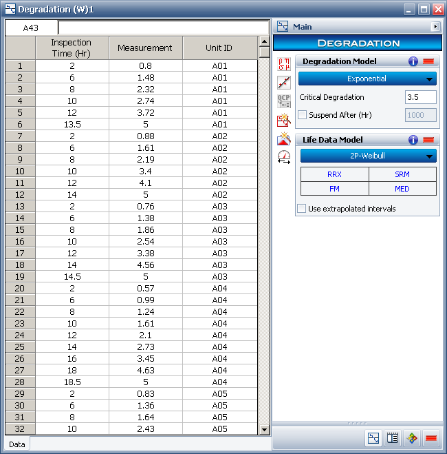
The first step in this analysis is to specify a degradation model to use to fit the observed data. For this type of failure mode, it was determined that the exponential degradation model is an appropriate model (the choice of degradation model comes from a physics of failure understanding of how the degradation of the performance/quality progresses over time). After the parameters of the degradation model are calculated for each of the observed units, the models can be used to estimate the times that correspond to the warning limit of thickness. This is done by setting the Critical Degradation field on the Main page of the control panel to 3.5. Using the fitted degradation model, the time values equivalent to the warning limit of thickness are calculated. (To see these time values, after calculating, click the ... icon in the Degradation Results area of the control panel and view the Extrapolated Failure-Suspension tab in the Results window.) A plot of degradation versus time with the failure thickness and warning limit labeled is shown next.

Table 1 summarizes the estimated "P" and "F" times in addition to the P-F interval or FDT values for each observed unit. The P-F interval or FDT values for each observed unit use the following equations:

P-F Interval = F P

FDT = P/F

Table 1: P and F results for each observed pipe along with the calculated P-F interval and FDT

Unit ID	Warning (P)	Failure Time (F)	P-F Interval	FDT
A01	11.33	13.5	2.17	0.84
A02	11.05	14	2.95	0.79
A03	12.19	14.5	2.31	0.84
A04	15.90	18.5	2.60	0.86
A05	13.34	15.7	2.36	0.85
		Average	2.48	0.84

 

The P-F interval and FDT average values shown above can be used as the final P-F interval and FDT estimates (you can also use median values).

Using P-F Interval and FDT in System Modeling

After estimating the P-F intervals or FDT values that describe the detectability of failures, the analyst can use either of these values to analyze a systems reliability and availability and/or to select the appropriate maintenance strategy for the equipment. Reliability centered maintenance (RCM) and system analysis using reliability block diagrams (RBDs) are two typical approaches for the analysis of repairable systems.

The next figures show how P-F intervals or FDT values can be specified in the properties of an on condition task, which can be used for repairable systems analysis in RCM++ or BlockSim.

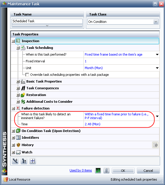
Note that on condition tasks include both an inspection portion, which dictates when the component or system will be inspected and uses either a P-F interval or FDT value to describe the detectability of failure, and a preventive portion, which specifies the preventive maintenance that occurs if and when it is triggered by the detection of failure during inspection.

Estimating Efficient Inspection Intervals

If inspections are done frequently, the costs due to inspections will be high, but so will be the likelihood of catching potential failures. On the other hand, if inspections are performed rarely, the costs due to inspections will be lower but so will be the likelihood of detecting potential failures. In practice, inspection intervals that are equal to half of the P-F interval are considered to be adequate. [1] The time necessary to take an action also needs to be considered to ensure that ample time is allocated for repairs. The severity of the failure also weighs into the decision on the frequency of the inspection interval.

BlockSim and RCM++ allow the analyst to evaluate the impact of the use of a certain inspection period on the component and the system. The impact can be described based on different criteria such as availability, throughput, uptime and profit. Various inspection intervals can be compared and the optimum inspection interval can be determined.

Conclusion

This article explained how the detectability of failures as expressed by P-F intervals or FDT can be estimated based on degradation data. It also showed how such information can be incorporated into repairable system analysis in BlockSim or RCM++.

References

1. Moubray, John, Reliability-Centered Maintenance, Industrial Press, Inc., New York City, NY, 1997.