Monitoring Warranty Returns Using Statistical Process Control (SPC)
Warranty return predictions are important for companies because they help create an idea about the anticipated number of returns for each subsequent period, determine whether improvements are necessary if the expected returns are too high and determine how many spare parts to manufacture, allocate or ship to distributors in order to be better prepared for quick customer warranty claims fulfillment.
Warranty return predictions can also be used as a tool to verify whether actual experienced returns fall in line with expectations. By monitoring warranty return data, the analyst (and the organization) can detect specific return periods and/or batches of sales or shipments that deviate from the assumed model by comparing actual returns to the previously predicted returns. If the actual experienced returns number deviates significantly from the number that was predicted, a flag would be raised calling for further investigations or for actions to be taken to treat the problem. This provides the advantage of early notification of possible deviations in manufacturing, use conditions and/or any other factors that may adversely affect the reliability of the fielded product. Obviously, the motivation for performing such analysis is to allow for faster intervention to avoid increased costs due to increased warranty returns or more serious repercussions.
This article will discuss a methodology for monitoring warranty returns using Statistical Process Control (SPC). It will not, however, discuss how warranty data sets are analyzed and how predictions are generated. For more information about warranty data analysis and returns prediction, click here.
Analysis Method
For each sales period i and return period j, the prediction error can be calculated as follows:

where
 is the estimated number of failures based on the estimated distribution
parameters for the sales period i and the return period j,
calculated using the model that was fitted to the warranty data. Fi,j
is the actual number of failures for the sales period i and
the return period j.
Since we are assuming that the model is accurate, ei,j should follow a normal distribution with a mean (ēi,j) value of zero and a standard deviation s:
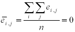

Where n is the total number of return data (total number of residuals).
ei,j can be normalized as follows:
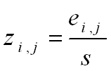
where zi,j is the standardized error. zi,j follows a standard normal distribution with μ = 0 and σ = 1.
It is known that the square of a random variable with standard normal distribution follows the χ2 (Chi-Square) distribution with 1 degree of freedom and that the sum of the squares of m random variables with standard normal distribution follows the χ2 distribution with m degrees of freedom. This then can be used to help detect the abnormal returns for a given sales period, return period or just a specific cell (a return piece of data which is defined by a combination of a specific return and a specific sales period).
For a cell, abnormality is detected if:

For an entire sales period i, abnormality is detected if:

where J is the total number of return periods for a sales period i.
For an entire return period j, abnormality is detected if:

where I is the total number of sales periods for a return period j.
Here, α is the criticality value of the χ2 distribution, which can be set at critical value or caution value. It describes the level of sensitivity to outliers (returns that deviate significantly from the predictions based on the fitted model). Increasing the value of α increases the power of detection, but this could lead to more false alarms.
Note: SPC calculations can be performed only under the Nevada format for warranty returns because it provides the convenient format for the required calculations. Weibull++ also provides the capability of converting other types of warranty return data to the Nevada format, which allows users who prefer other types of warranty data entry to convert their data to the Nevada chart and perform the SPC analysis. For details about warranty data conversion, please refer to the Weibull++ manual or the help file in Weibull++.
Example 1
Let us consider the following warranty data.

Using the MLE analysis method and assuming a Weibull distribution, the estimated parameters are β = 2.4928, η = 6.6951.
The expected returns for each sales period can be obtained using conditional reliability concepts. For example, for the third return month of the first sales period, the expected return number is given by:

The actual returns in this period were five, thus the prediction error for this period is:

This can then be repeated for each cell, yielding to the following table for ei,j :

Now, for this example, n = 6, ēi,j = −0.5432 and s = 1.6890.
Thus the zi,j values are:

The z2i,j(χ21) values, for each cell, are given in the following table.

If the critical value is set at α = 0.01 and the caution value is set at α = 0.1, then the critical and caution χ2 values will be:

If we consider sales periods as the basis for outlier detection, then after
comparing the above table to the sum of z2i,j(χ21)
values for each sales period, we find that none of the sales values
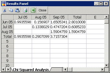
exceed the critical and caution limits. For example, the total χ2 value of the sale month of July is 0.6085. Its degrees of freedom is 2,
so the corresponding caution or critical values are 4.6052 and 9.2103
respectively. Both values are larger than 0.6085, so the return numbers of
the July sales period do not deviate (based on the chosen significance) from
the models predictions.
If we consider returns periods as the basis for outliers detection, then after comparing the above table to the sum of z2i,j(χ21) values for each return period, we find that none of the return values exceed the critical and caution limits. For example, the total χ2 value of the sale month of August is 3.7157. Its degree of freedom is 3, so the corresponding caution and critical values are 6.2514 and 11.3449 respectively. Both values are larger than 3.7157, so the return numbers for the June return period do not deviate from the models predictions.
The above analysis can be automatically performed in Weibull++ by entering the alpha values on the SPC tab and selecting what type of color code to use under Color Code Returns Sheet.
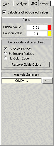
The Chi Squared values ( z2i,j or χ21 values) can be seen in the next figure (obtained by clicking the Show Analysis Summary(...) button on the SPC tab).
Weibull++ automatically color codes SPC results for easy visualization in the returns data sheet. By default, the green color means that the return number is normal; the yellow color indicates that the return number is larger than the caution threshold but smaller than the critical value; the red color indicates that the return is abnormal, meaning that the return number is either too large or too small compared to the predicted value.
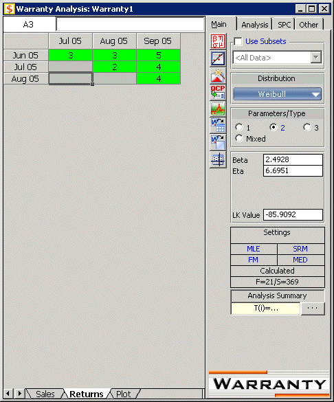
In this example, all the cells are coded in green for both analyses,By Sales Periods and By Return Periods, indicating that all returns fall within the caution and critical limits (i.e. nothing is abnormal). Another way to visualize this is by using a Chi-Square plot as shown in the next two figures.
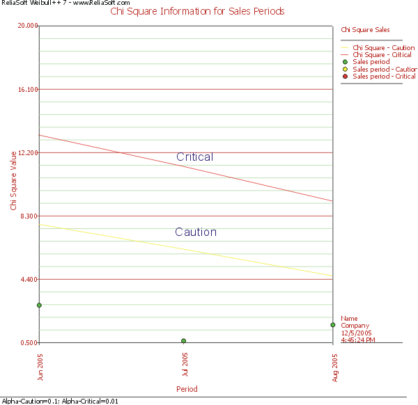
The Chi-Square plot for sales is:
The Chi-square plot for returns is:
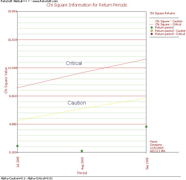
As can be seen in these two plots, all return data fall under the caution and critical lines, assuring that the returns are statistically normal.
Example 2
A manufacturer collects the following sales and return data.

The data set is analyzed using the two-parameter Weibull distribution and the MLE analysis method. The parameters are estimated to be β = 2.31 and η = 25.07.
The SPCs α values are set at 0.01 for the Critical Value and 0.1 for the Caution Value. When analyzed and color coded in Weibull++, the following window is obtained.
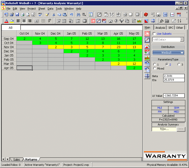
Here the Nov. 04 and Mar 05 sales periods are colored in yellow indicating that they are outlier sales periods that the manufacturer needs to be cautioned about, while the rest are green.
The manufacturer wants to find the root cause for the variation of the Nov 04 and Mar 05 in comparison with the other production periods. Further investigations show that there were variations in the material used in production during the two periods of concern. For these periods, the material used was acquired from a different supplier. This implies that the units are not homogeneous, and that there are different subpopulations present in the field populations.
Based on this, the data set is re-analyzed after categorizing the different shipments (using the ID column) based on their material supplier. The data are entered as shown next.
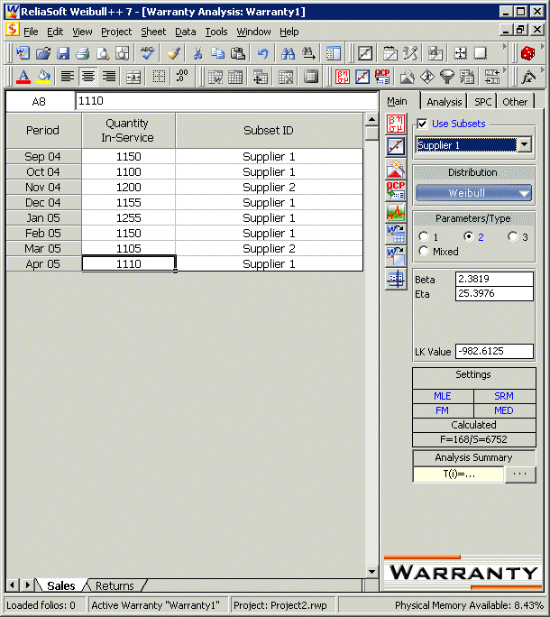
Each subset of data (supplier 1 and supplier 2) is analyzed separately. The new models that describe the data are (assuming a two-parameter Weibull distribution and using MLE as the analysis method for both sub-populations):
| Supplier 1 | Supplier 2 |
| β = 2.38 | β = 2.32 |
| η = 25.39 | η = 21.28 |
This analysis helped in uncovering different subpopulations as well as allowing us to compute different distributions for each subpopulation. Note that if the analysis were performed on the failure and suspension times in a regular Standard Folio, using the mixed Weibull distribution, one would not be able to detect which units fall into which subpopulation.