Modeling Interactions Between Variables in Accelerated Life Testing or Life-Stress Analysis
[Editor's Note: This article has been updated since its original publication to reflect a more recent version of the software interface.]
When analyzing accelerated test life data or life-stress data, interactions between factors are often wrongly ignored or poorly understood and yet have significant impact. This article presents a simple methodology for analyzing the significance of interactions among different factors and incorporating their effects into the reliability analysis.
Example
A paper manufacturer is investigating the effect of the percentage of hardwood concentration in raw pulp, the vat pressure and the cooking time of the pulp on the strength of paper. A life-stress experiment was conducted to assess the strength of the paper and the data set presented in Figure 1 was collected. The manufacturer wants to find the optimum settings for the production factors that result in a desirable paper strength.
Note: In addition to being an accelerated life data analysis software, Accelerated Life Testing PRO can be used to analyze life-stress relationships similar to Design of Experiments (DOE) tests analyzed with various DOE software packages. The advantage of using Accelerated Life Testing PRO for this type of analysis is the ability to involve life distributions and to use physical properties knowledge to relate the stress variables to the life (or other characteristics) of the product. In this example, the paper (produced under different settings) is put under test (normal conditions) and the strength of the paper is recorded.
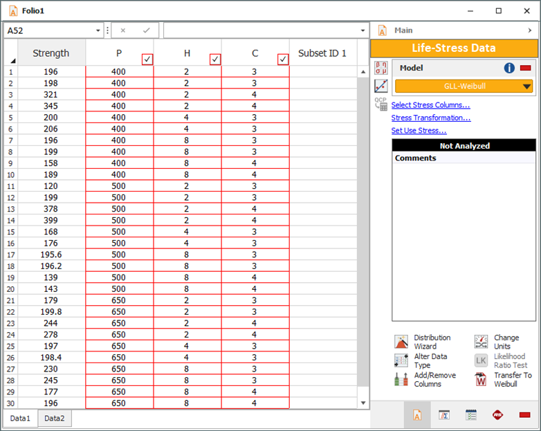
Figure 1: Test results
for paper strength as a factor of the different production variables
Because this is a multivariate test example, the General Log-Linear model can be used to analyze the data. (Note that the General Log-Linear model is available only in Accelerated Life Testing PRO, not in Accelerated Life Testing Standard.) From the equation of the General Log-Linear model, we obtain the following.
![]()
where:
- α0, α1, α2 , α3, α4, α5, α6, α7 are model parameters.
- X1(lb/in2) represents the Pressure (P) variable.
- X2(%) represents the Hardwood Concentration (H) variable.
- X3(h) represents the Cooking Time (C) variable.
- X4 = X1X2 represents the Pressure/Hardwood Concentration interaction term.
- X5 = X1X3 represents the Pressure/Cooking Time interaction term.
- X6 = X2X3 represents the Hardwood Concentration/Cooking Time interaction term.
- X7 = X1X2X3 represents the Pressure/Hardwood Concentration/Cooking Time interaction term.
- X is a vector of n (n=7) stresses.
- L(X) is the expected strength.
In Accelerated Life Testing, additional columns representing the interaction term are required. In this example, the interaction columns are obtained through the multiplication of the stress values of the interaction term's variables. For example, for the X1X2 (PH) interaction term, the interaction column is to be filled by multiplying the values of the P and C columns. With the interaction columns, the data sheet looks like the one shown next.

First, choose Life-Stress Data > Options > Select Stress Columns and include all the terms in the analysis, as shown next.

Click Stress Transformation directly underneath the Model area of the Main page of the control panel, and define the stress relationships as follows.

Using Weibull as the life distribution, the parameter values with 80% two-sided confidence are:
|
Lower = -1.5203 |
α0 = 0.5216 |
Upper = 2.5635 |
|
Lower = 0.0002 |
α1 = 0.0041 |
Upper = 0.0080 |
|
Lower = 0.2179 |
α2 = 0.5247 |
Upper = 0.8314 |
|
Lower = 1.0124 |
α3 = 1.6543 |
Upper = 2.2961 |
|
Lower = -0.0008 |
α4 = -0.0002 |
Upper = 0.0003 |
|
Lower = -0.0028 |
α5 = -0.0015 |
Upper = -0.0003 |
|
Lower = -0.2892 |
α6 = -0.1962 |
Upper = -0.1032 |
|
Lower = -4.7422E-5 |
α7 = 0.0001 |
Upper = 0.0003 |
This table shows that the 80% bounds on α4 and α7 include 0, therefore the X1X2 (PH), X1X2X3 (PHC) interaction terms can be ignored. The analysis is repeated without these terms, as shown next.

The new model is:
![]()
where:
- X1(N) represents the Pressure (P) variable.
- X2(%) represents the Hardwood Concentration (H) variable.
- X3(h) represents the Cooking Time (C) variable.
- X4 = X1X3 represents the Pressure/Cooking Time interaction term.
- X5 = X2X3 represents the Hardwood Concentration/Cooking Time interaction term.
The new 80% bounds on the parameter values are:
| Lower = 1.3154 | α0 = 2.1284 | Upper = 2.9413 |
| Lower = -0.0009 | α1 = 0.0008 | Upper = 0.0024 |
| Lower = 0.3624 | α2 = 0.4264 | Upper = 0.4905 |
| Lower = 0.7485 | α3 = 0.9908 | Upper = 1.2330 |
| Lower = -0.0007 | α4 = -0.0002 | Upper = 0.0003 |
| Lower = -0.1540 | α5 = -0.1358 | Upper = -0.1176 |
This table shows that the 80% bounds on α1 and α4 include 0, therefore the X1 (P) and the X1X3 (PC) interaction term can be ignored. The analysis is repeated without these terms.

The new model is:
![]()
where:
- X1(%) represents the Hardwood Concentration (H) variable.
- X2(h) represents the Cooking Time (C) variable.
- X3 = X2X3 represents the Hardwood Concentration/Cooking Time interaction term.
The new 80% bounds on the parameter values are:
| Lower = 2.1378 | α0 = 2.4718 | Upper = 2.8058 |
| Lower = 0.3804 | α1 = 0.4406 | Upper = 0.5009 |
| Lower = 0.8127 | α2 = 0.9093 | Upper = 1.0059 |
| Lower = -0.1564 | α3 = -0.1392 | Upper = -0.1220 |
None of the above bounds include 0, therefore all the included terms are considered to be significant.
The following figure displays the Standardized vs. Fitted Value Residuals plot. It shows no obvious abnormality, which confirms that the new model is valid.

The purpose of this experiment is to determine the settings that produce a paper strength greater than 200. The estimated percentage of population with a strength greater than 200 is calculated at different settings of Hardwood Concentrations and Cooking Times. This is performed using the Quick Calculation Pad (QCP), varying the values of the variables and the associated interaction term and setting Mission End Time at 200.

The following table summarizes the results.

Therefore, the optimum settings for the production factors are found to be at Cooking Time = 4 hr and Hardwood Concentration = 2%. Under these conditions, 99.98% of the paper produced will have a strength greater than 200.