Data Analysis and Reporting

The manner in which reliability data is analyzed and reported will largely have to be tailored to the specific circumstance or organization. However, it is possible to break down the general methods of analysis/reporting into two categories: non-parametric analysis and parametric analysis. Overall, it will be necessary to tailor the analysis and reporting methods by the type of data as well as to the intended audience. Managers will generally be more interested in actual data and non-parametric analysis results, while engineers will be more concerned with parametric analysis. Of course this is a rather broad generalization and if the proper training has instilled the organization with an appreciation of the importance of reliability engineering, there should be an interest in all types of reliability reports at all levels of the organization. Nevertheless, managers are usually more interested in the "big picture" information that non-parametric analyses generally tend to provide, while not being particularly interested in the level of technical detail that parametric analyses provide. On the other hand, engineers and technicians are usually more concerned with the close-up details and technical information that parametric analyses provide. Both of these types of data analysis have a great deal of importance to any given organization, and it is merely necessary to apply the different types in the proper places.

Non-Parametric Analysis

Data conducive to non-parametric analysis includes information that has not or cannot be rigorously processed or analyzed. Usually, it is simply straight reporting of information, or if it has been manipulated, it is usually by simple mathematics, with no complex statistical analysis. In this respect, many types of field data lend themselves to the non-parametric type of analysis and reporting. In general, this type of information will be of most interest to managers as it usually requires no special technical know-how to interpret. Another reason it is of particular interest to managers is that most financial data falls into this category. Despite its relative simplicity, the importance of non-parametric data analysis should not be underestimated. Most of the important decisions that are made concerning the business are based on non-parametric analysis of financial data.

As mentioned in last month's issue of the HotWire ("Data Collection"), ReliaSoft's Dashboard system is a powerful tool for collecting and reporting data. It especially lends itself to non-parametric data analysis and reporting, as it can be quickly processed and manipulated in accordance with the user's wishes.

Non-Parametric Reliability Analysis

Although many of the non-parametric analyses that can be performed based on field data are very useful for providing a picture of how the products are behaving in the field, not all of this information can be considered "hard-core" reliability data. As was mentioned earlier, many such data types and analyses are just straight reporting of the facts. However, it is possible to develop standard reliability metrics, such as product reliability and failure rates, from the non-parametric analysis of field data. A common example of this is the "diagonal table" type of analysis that combines shipping and field failure data in order to produce empirical measures of defect rates.

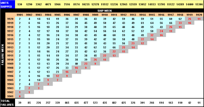
Table 1 gives an example of a "diagonal table" of product shipping and failure data by shipment week. The top row, highlighted in blue and yellow, shows the number of units of product that were shipped in a given week, labeled from 9901 to 9920. The data highlighted in blue and gray represents the number of units that were reported failed or had warranty hits in the subsequent weeks after being shipped. This information can be used to calculate a simple percent defective for each shipment week. Note that one must make certain to use a weighting factor to account for the amount of time a particular week's worth of units have spent in the field. Also, care should be taken to account for the delay between shipping and actual installation, which can be a substantial time period for some products. The time period for the average delay (in this example, two weeks, which is highlighted in gray in the table) should be removed from the data being analyzed. Otherwise, a false appearance of a decreasing defect rate appears in the final results of the analysis. Figure 1 shows the results of the non-parametric defect rate calculation, unadjusted and adjusted for the two-week average delay between shipping and installation.

Table 1: Diagonal table of field data for non-parametric analysis [CLICK TO ENLARGE]

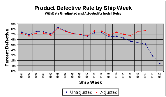
Figure 1: Percent defective results for data in Table 1, unadjusted and adjusted for installation delay

Parametric Analysis

Data that lends itself to parametric statistical analysis can produce very detailed information about the behavior of the product based on the process utilized to gather the data. This is the "hard-core" reliability data with all the associated charts, graphs and projections that can be used to predict the behavior of the products in the field.

The origin of this type of data is usually in-house, from reliability testing done in laboratories set up for that specific purpose. For that reason, a great deal more detail will be associated with these data sets than with those that are collected from the field. Unfortunately, when dealing with field data, it is often a matter of taking what you can get, without being able to have much impact on the quality of the data. Of course, setting up a good program for the collection of field data will raise the quality of the field data collected, but generally it will not be nearly as concise or detailed as the data collected in-house.

The exception to this generalization is field data that contains detailed time-of-use information. For example, automotive repairs that have odometer information, aircraft repairs that have associated flight hours or printer repairs that have a related print count can lend themselves to parametric analysis. Caution should be exercised when this type of analysis is performed, however, to make sure that the data are consistent and complete enough to perform a meaningful parametric analysis.

Although it is possible to automate parametric analysis and reporting, care should be taken in automatic processing. Caution is required because of the level of detail inherent in this type of data and the potential "disconnect" between field data and in-house testing data (described in "Field Data"). Presentations of these two types of data should be carefully segregated in order to avoid unnecessary confusion among the end users of the data reports. It is not unusual for end users who are not familiar with statistical analysis to become confused and indignant when presented with seemingly contradictory data on a particular product. The tendency in cases such as these is to accuse one or both sources of data (field or in-house) of being inaccurate. This is, of course, not necessarily true. There will usually tend to be a disparity between field data and in-house reliability data.

Another reason for the segregation of the field data and the in-house data is the need for human oversight when performing the calculations. Field data sets tend to undergo relatively simple mathematical processing that can be safely automated without having to worry about whether the analysis type is appropriate for the data being analyzed. However, this can be a concern for in-house data sets that are undergoing a more complicated statistical analysis. This is not to say that parametric analysis should not be in any way automated. However, a degree of human oversight should be included in the process to insure that the data sets are being analyzed in an appropriate manner. Furthermore, the data should be cross-referenced against the Test Log and Service Log to make sure that irrelevant or "outlier" information is not being included in the data.

Examples of Reporting for Parametric Data Analysis

Following are some examples of the information that can be generated using parametric data analysis. While this is by no means complete, it serves as a starting point for the information that can be obtained with the proper collection of data and parametric analysis.

Probability Plot

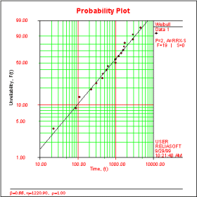
Probability plotting was originally a method of graphically estimating distribution parameter values. With the use of computers that can precisely calculate parametric values, the probability plot now serves as a graphical method of assessing the goodness of fit of the data to a chosen distribution. Probability plots have nonlinear scales that will essentially linearize the distribution function, and allow for assessment of whether the data set is a good fit for that particular distribution based on how close the data points come to following the straight line. The y-axis usually shows the unreliability or probability of failure, while the x-axis shows the time or ages of the units. Specific characteristics of the probability plot will change based on the type of distribution.

Reliability Function

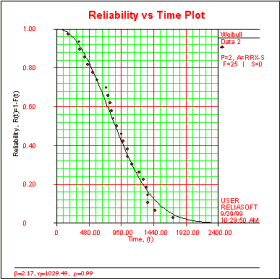
The reliability function gives the continuous probability of a successful mission versus the time of the mission. This is similar to the probability plot in that it shows the performance of the product versus the time. However, it does not have nonlinear scales on the axes and the y-axis gives the reliability instead of the unreliability.

Probability Density Function

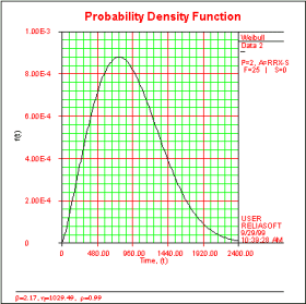
The probability density function (pdf) represents the relative frequency of failures with respect to time. It basically gives a description of how the entire population from which the data is drawn is spread out over time or usage. The probability density function is most commonly associated with the "bell curve," which is the shape of the pdf of the normal or Gaussian distribution.

Failure Rate Function

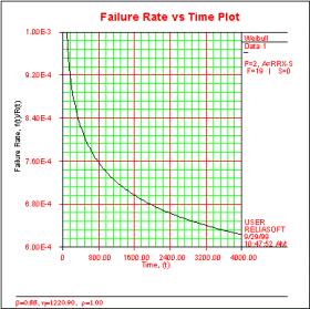
The failure rate function indicates how the number of failures per unit time of the product changes with time. This provides a measure of the instantaneous probability of product failure changes as usage time is accumulated. The failure rate plot is associated with the "bathtub curve," which is an amalgamation of different failure rate curves to illustrate the different ways in which products exhibit failure characteristics over the course of their lifetimes.

Likelihood Function

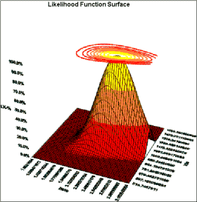
The likelihood function is a more esoteric function of the data, but it is directly related to how the parameters are calculated. The likelihood function relates the data points to the values for the parameters of the distribution. The maximization of this function determines the best values for the distribution's parameters.

Life vs. Stress Plot

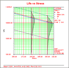
The Life vs. Stress plot is a product of accelerated life testing or reliability testing that is performed at different stress levels. This indicates how the life performance of the product changes at different stress levels. The gray shaded areas are actually pdf plots for the product at different stress levels. Note that it is difficult to make a complete graphical comparison of the pdf plots due to the logarithmic scale of the y-axis.

Reliability Importance

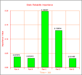
Reliability importance is a measure of the relative weight of components in a system, with respect to the system's reliability value. The higher the reliability importance a particular component has, the larger the effect that component has on the system's reliability. This measure is useful in helping to optimize system reliability performance, as it helps to identify which components will have the greatest effect on the overall system reliability.

Reliability Growth

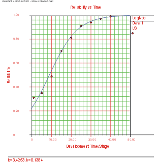
Reliability growth is an important component of a reliability engineering program. It essentially models the change in a product's reliability over time and allows for projections on the change in reliability in the future based on past performance. It is useful in tracking performance during development and aids in the allocation of resources. There are a number of different reliability growth models available that are suitable to a variety of data types. The above chart is a graphical representation of the logistic reliability growth model.