Determining Reliability for Complex Systems
Part 2 - Simulation

In the previous article, we discussed methods to analytically determine the reliability of a complex system. While the analytical method has a number of advantages, such as being able to determine the pdf or the failure rate for the entire system, there are also some drawbacks. A major disadvantage of analytical analysis of complex systems is the complexity of the solutions. Calculating the analytical reliability solution for a sizable complex system may tax the resources of even the most powerful PC. In situations such as this, it may be more advantageous to use simulation to determine the complex system's reliability. This article discusses the methodology used by ReliaSoft BlockSim to simulate system reliability. (NOTE: you may want to download a free evaluation version of BlockSim in order to perform some of the following examples.)

A complex system is one that cannot be broken down into groups of series and parallel components. In many cases it is not easy to recognize which components are in series and which are in parallel in a complex system. The following network is a good example of such a complex system:

As the figure illustrates, this system cannot be broken down into a group of series and parallel systems. If the system can be broken down into series/parallel configurations, it is a relatively simple matter to determine the mathematical or analytical formula that describes the system's reliability. However, for a complex system, determination of the system reliability becomes more involved.  

In this article, we will look at some of the techniques that can be employed to determine a system's reliability via simulation. It is assumed that the reliability values for the components have been determined using standard (or accelerated) life data analysis techniques, so that the reliability function for each component is known. With this component-level reliability information available, simulation can then be performed to determine the reliability of the entire system.  

Monte Carlo Simulation

Simulation in system reliability analysis is based on the Monte Carlo simulation method that generates random failure times from each component's failure distribution. The overall system reliability is then obtained by simulating system operation and empirically calculating the reliability values for a series of time values. Through the use of computers, simulation has become a very popular analysis tool. Simulation is simple to apply and it can produce results that can be rather difficult to solve analytically. On the other hand, simulation methods also have certain drawbacks, not the least of which is that the results depend on the number of simulations, which results in a lack of repeatability. Other drawbacks are that systems with static components (i.e., components in which the reliability does not change with time) cannot be simulated, and that most of the reliability optimization and allocation techniques cannot be applied.

To illustrate how Monte Carlo data points are generated, we will demonstrate how to generate times to failure based on a two-parameter Weibull distribution with beta equal to two ( =2) and eta equal to 100 (=100). The reliability equation for the two-parameter Weibull distribution is given by:

where 0 < R(T) < 1. If we assume that the values of R(T) are uniformly distributed over the interval between 0 and 1, then we can let U, a uniformly distributed random number in the same interval, represent R(T). Substituting U for R(T), beta (), eta (), and solving for T yields:

This equation is valid for any uniform random number U, 0 < U < 1. The procedure is then repeated using newly generated random numbers, U, until the desired number of simulated failure times, T, are reached.

The same methodology, using different equations, is used for other distributions.

System Simulation Methodology

The system simulation methodology process is based on the Monte Carlo simulation method which was described in the previous section. This is different from the analytical methodology discussed in last month's issue. While one can perform a Monte Carlo simulation based on the results of the analytical system reliability solution, this should not be confused with the methodology described below, which uses Monte Carlo simulation of the individual components to estimate the overall system reliability.

In BlockSim, the reliability simulation option requires a number of inputs. The first input is the end time at which the reliability is to be estimated. The second input is the number of increments. The end time is divided into the number of increments specified. When the simulation is performed, a table of reliabilities and instantaneous failure rates is generated for each incremental time up to the end time. However, only the instantaneous failure rate estimation is affected by the number of increments. The Use Seed option allows the user to choose the seed value for the generation of random numbers. Use of the same seed value will result in identical simulation results, provided the other inputs remain the same.

The next two inputs for the simulation, the number of inner loops and the number of outer loops, can be found on the Setup page of the Reliability/Maintainability Simulation window. The product of the two values will determine the total number of simulations to be performed. The number of inner loops indicates the number of simulation points to be generated for each component. The number of outer loops indicates the number of repetitions of the inner loops. If, for example, 1000 inner loops and 10 outer loops are to be performed, this means that first 1000 simulation points will be generated and the reliability of the system at the end of each of the 1000 runs will be calculated. This will then be repeated 10 times, each time with a new stream of random numbers for the simulation points. This will yield 10 different system reliability values each obtained from 1000 runs. The average of these 10 reliability values will be the returned system reliability at the specified time.

In summary, the simulation procedure consists of the following steps:

• Step 1 - Decide on the number of points to generate (Inner Loops).

• Step 2 - For each run, generate a random number between 0 and 1.

• Step 3 - Obtain a failure time for each component based on this random number.

• Step 4 - Keep the smallest time-to-failure with the corresponding component (i.e., time-to-failure with a value less than the desired mission time).

• Step 5 - Check which components or combination of components cause system failure.

• Step 6 - The unreliability of the system is the number of times the system was found to have failed divided by the total number of runs. The reliability of the system is 100% minus the unreliability.

• Step 7 - Return to Step 2 and repeat the procedure for the desired number of cycles (Outer Loops).

• Step 8 - The reliability of the system is the summation of the reliabilities of the Outer Loops divided by the number of Outer Loops (i.e., the average reliability).

BlockSim System Simulation Example

In order to illustrate these principles, consider the following complex system:

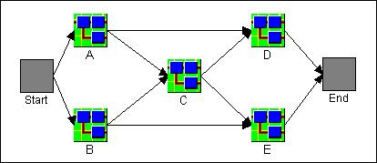
Given that components A through E are identical, with a two-parameter Weibull failure distribution with a beta value of 1.2 ( =1.2) and an eta value of 1230 ( =1230), determine the reliability of the system at 1500 hours. Note that the Start and End blocks cannot fail. The Reliability/Maintainability Simulation utility in BlockSim is used for this example. Since we are not solving for system reliability using analytical techniques, the reliability equation for the system cannot be obtained. However, a table of reliability vs. time can be generated. First, open the Reliability/Maintainability Simulation window. On the Reliability page, enter an End Time of 1500 hrs, 15 Increments, and a Seed Value of 1. When you perform the simulation, these settings will generate a table of 15 reliability values with the corresponding times and failure rates.

On the Setup page of the Reliability/Maintainability Simulation window, specify 5 Outer Loops and 10,000 Inner Loops.

This means that 10,000 random times-to-failure will be generated for each component. This failure time will be compared to the simulation time increment. If the failure time is less than the time increment, a failure will be counted against the system. The system reliability is the ratio of the number of successes to the number of trials (in this case, there are 10,000 trials). The process is repeated 5 times, and the results averaged to get a system reliability value at each time increment. When the simulation is complete, the Results Panel window will appear with the corresponding results.

As you can see from the preceding table, the reliability of the system at 1500 hours is 0.1738, or 17.38%. This gives a simple demonstration of how system reliability simulation works. While the technique is rather simple, it also requires many repetitions in order to develop a realistic solution, thus making the use of a computer necessary to be able to perform the analysis in a timely fashion.  

In future issues of the Reliability HotWire, we will look at how simulation can be used to determine a system's availability as well as its reliability.