Using Markov Diagrams in BlockSim for Availability Analysis

In the November 2015 issue of Reliability HotWire, the Hot Topics article included a discussion on Markov chains and went through the methodology of how to use a discrete Markov chain in BlockSim in order to analyze a system that can be in several different states of usage or decay. In this issue, we will describe continuous Markov chains and present a methodology to use them for availability estimations for a system (if this feature is supported by your BlockSim license).

The main difference between a discrete Markov chain and a continuous Markov chain is that the transitions between the states are no longer represented by a fixed probability per step, but instead with a transition rate (constant) per unit time.

Because the transitions between states are represented by transition rates, the probability of being in a given state at a given time is represented by a differential equation for each state:

where:

• n is the total number of states
• Pj is the probability of being in state j
• Pl is the probability of being in state l
• λlj is the transition rate from state l to state j
• λjl is the transition rate from state j to state l

The initial probabilities of the states represent the initial conditions used to solve the system of differential equations.

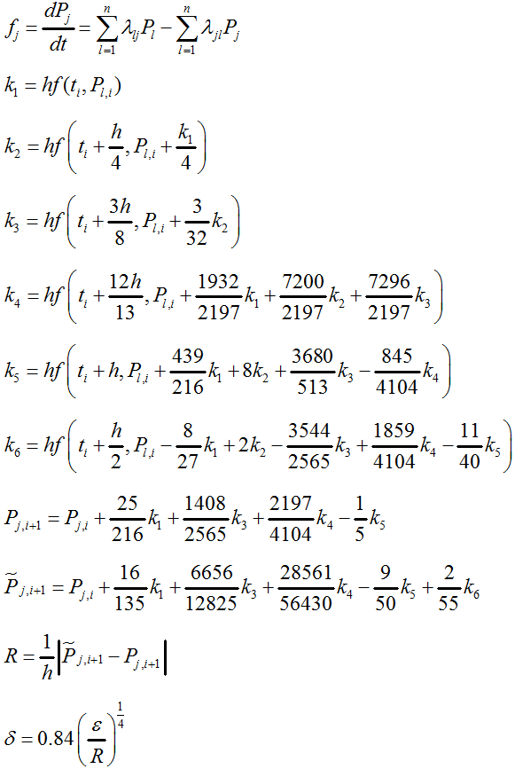
There are many different numerical methodologies to solve systems of differential equations. ReliaSoft chose to use a slightly modified version of the Runge-Kutta-Fehlberg method, the RKF45 method. This methodology is preferred as it allows for error estimations during calculations which, in turn, give us the power of an adaptive step size. The adaptive step size allows for faster calculations when the transition rates are small, and more accurate calculations when the transition rates are high, compared to a method that uses a fixed step size.

The method itself is basically a combination of a 4th order and a 5th order Runge-Kutta where the 4th order is used for the actual calculations and the 5th order is used to estimate error, and therefore adapt step size if needed:

If R ≤ ε then keep Pi+1 as the current solution, and move to the next step with step size δh; if R > ε then recalculate the current step with step size δh.

Where:

• Pj is the probability of being in state j
• Pl,i is the probability of being in state l at time i
• λlj is the transition from state l to state j
• λjl is the transition from state j to state l
• fj is the change in the probability of being in state Pj (note that fj is not a function of time for constant transition rate Markov chains)
• h is the time step size
• ti is the time at step i
• ε is the chosen acceptable error

After calculating all the probabilities of being in each state in the time frame desired, we can use those probabilities to estimate system availability, reliability and even system costs if the states are associated with a cost per unit time.

Example

Assume that we have a system which can go through a degraded operational state between its fully operational state and its non-functional (unavailable) state (3 states total).

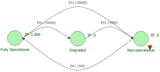
The system always starts in the fully operational state, as it is initially installed and begins operation. There is a chance that the system goes directly from fully operational to non-operational; and once non-operational, the system is restored back to fully operational. The transition rates between the states are:

• Fully Operational to Degraded has a transition rate with a mean time of 10,000 hours.
• Fully Operational to Non-operational has a transition rate with a mean time of 30,000 hours.
• Degraded to Non-operational has a transition rate with a mean time of 1,000 hours.
• Restoration from Non-operational to Fully Operational has a transition rate with a mean time of 500 hours.

We would like to estimate the time that the system spends in each state and the overall availability of the system over a 5 year period.

To help us solve this problem without having to do all the calculations by hand, we create a continuous Markov diagram in BlockSim. We first build our system, which is comprised of the 3 states and the transitions between them:

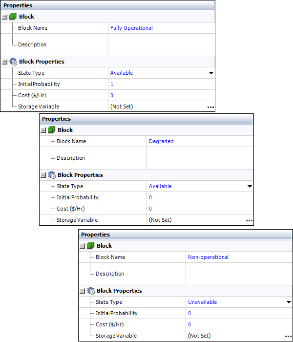
The states have the following properties:

The transition matrix looks like this (in events per hour):

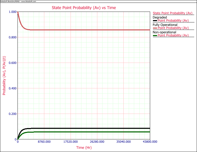
After we calculate the diagram for the 5-year interval, we use the point probability plot to see the probability of being in each of the 3 states at any given time:

We then check the results summary to determine the mean probabilities in each state and the point probabilities after 5 years:

From this, we calculate that the system has an availability of 0.944 (1 – 0.056), and we see that the system will spend 4.3 years in the fully operational state, 0.42 years in the degraded state and 0.28 years in the non-operational state.

Conclusions

In this article we examined the basic mathematical principles and practical applications of continuous Markov chains for system availability analysis. We then presented an example to show how you can use Markov chains to consider additional states other than fully operational and non-operational. When the information on the additional states is available, continuous Markov chains provide an alternative to the standard availability calculations.