Sensitivity Analysis Using Simulation Worksheets in BlockSim and DOE++
The combination of simulation methods and reliability block diagrams (RBDs) in reliability and maintainability analysis provides a powerful tool for estimating different system performance metrics (such as availability, maintenance costs, throughput, etc.) and identifying areas of improvement. A great benefit of this methodology is that it can then be used to perform sensitivity analysis in order to investigate the effect of different design options or maintenance policies on system performance. This article will illustrate how simulation worksheets in BlockSim can be used for this purpose.
Simulation worksheets allow the user to perform sensitivity analysis by varying multiple variables used in simulating a reliability block diagram (RBD) and investigating their effect on the simulation results. Some of the variables that can be used in the sensitivity analysis are listed next. (A complete list is available here.)
- Time interval of scheduled tasks
- Restock frequency in spare part pool
- Restock amount in a spare part pool
- Stock level that will trigger a restock in a spare part pool
- Number of simultaneous tasks a crew can perform
Once the variables of interest have been selected, one can either a) manually create a table with combinations of these variable levels in BlockSim or b) use DOE++ to design an experiment and transfer the design's variable combinations to BlockSim. Then a batch simulation of all the unique combinations can be performed and the results of interest (either at the system or block level) calculated. In this article, we will illustrate this process with the use of a simple example.
Example
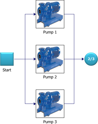
A reliability engineer is designing a system of three pumps in parallel, where at least two are required to operate at all times. Prior use of similar pumps in a different system has provided the engineer with the required failure and downtime distributions for the analysis. What she wants to determine in this case is the appropriate sparing strategy that will maximize the availability of the system while keeping maintenance cost at an acceptable level.
An RBD representing the reliability-wise configuration of the pumps is shown next.
The following figures show the reliability and maintenance properties for the pumps (all three have the same properties) and the spare part pool properties.
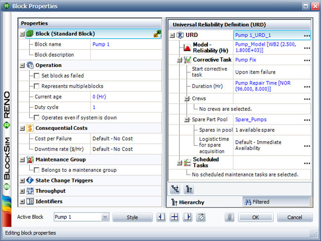
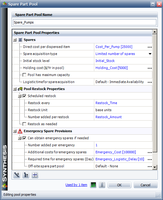
These properties show that each pump in stock has an associated acquisition and holding cost. If a spare pump is not available when needed, an emergency spare can be ordered for an additional cost and logistic delay. Based on past sparing policies, the initial stock is set to 1 pump and the spare pool is restocked every 3 months with 1 additional pump.
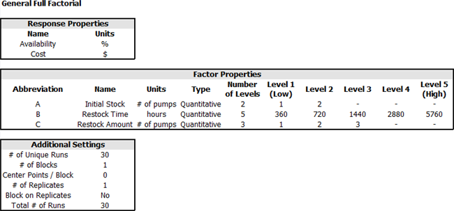
Given these properties, the system is simulated for 5 years of operation. The mean availability is found to be 95.0324% and the total maintenance cost is $6,572,565. As stated earlier, the reliability engineer wants to investigate whether a different sparing policy will yield a higher availability at a lower cost. In order to do this, she decides to use the simulation worksheet feature in BlockSim. The variables that will be included in this analysis are the initial stock level (1 or 2 pumps), the restocking frequency (2 weeks, 1 month, 2 months, 3 months or 4 months) and the amount that is restocked (1, 2 or 3 pumps).
In order to create combinations of these variables that can then be used to run simulations, the engineer designs a general full factorial experiment in DOE++. The design settings used in the standard folio are shown next.
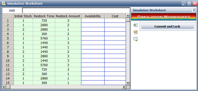
The next figure shows the simulation worksheet that contains all the unique combinations between initial stock level, restock time and restock amount.
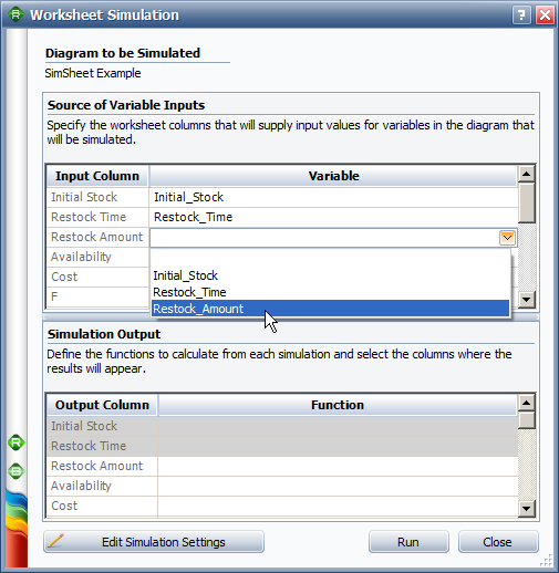
The next step is to assign the worksheet columns to the input variables that will be used in simulation. The next figure shows how to assign the columns to the variables that will be varied when simulating the RBD.
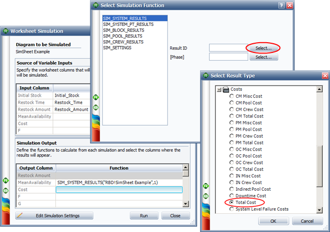
With respect to the calculated outputs, any simulation result can be used, either at the system or the block level. In this case the desired outputs were system mean availability and system total costs. The following figure shows the selection of system mean availability as one of the outputs.
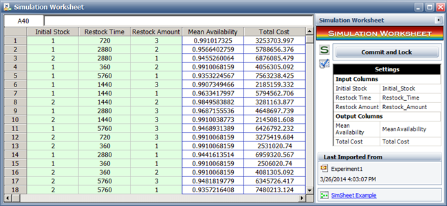
Given those settings, BlockSim can now simulate each combination of the three variables and estimate the corresponding mean availability and total costs over 5 years of operation, as shown next.
These results are now transferred back to the DOE++ folio for analysis. The following figure shows the resulting ANOVA table, using availability as the response. (More information about general full factorial designs is available here.)
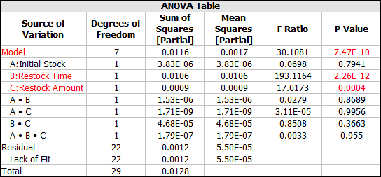
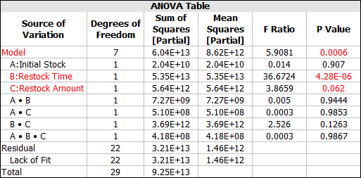
As shown in the table, only the restock time and the restock amount have a significant effect on system availability, while the initial stock level does not seem to be significant. The same conclusions are drawn when using cost as a response instead of availability, as shown next.
The last step is to identify the variable levels that will produce the maximum availability while keeping cost at a minimum. This can be done by either sorting the rows in the DOE++ folio in order to determine which combinations lead to an acceptable availability with the lowest cost, or by using optimization in DOE++. The following figure shows the calculated optimal solution in DOE++. (The factor values were treated as qualitative to ensure that the optimal settings match a combination used during simulation.)
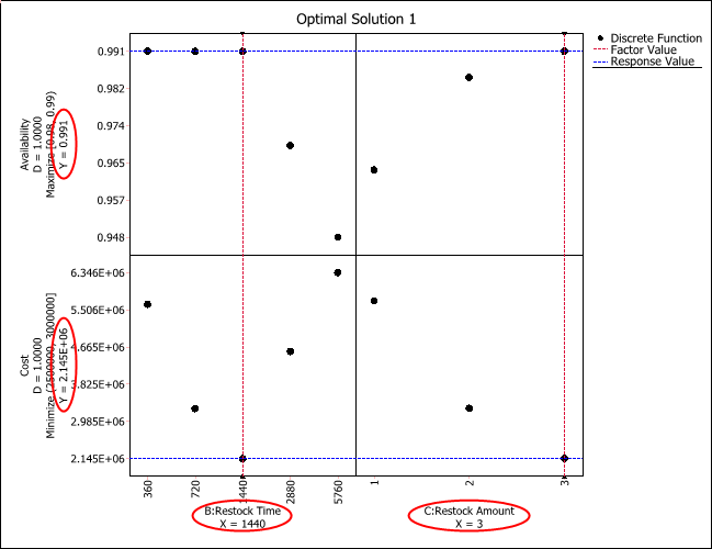
Note that the initial stock amount was excluded from this analysis because it was not found to be significant. As shown in the optimal solution plot, the suggested restock time is 1,440 hours (or 2 months), and the restock amount is 3 pumps. With these settings, the system availability is expected to be 99.1% (compared to 95.0324% with the original settings) and the total costs $2,145,000 (compared to $6,572,565).
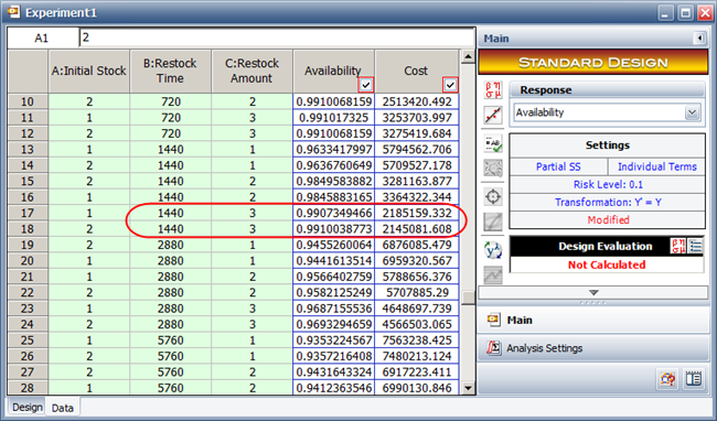
Finally, the model created in DOE++ might not produce the same results as BlockSim, depending on the relationship between the factors and response. Therefore, the optimum results calculated in DOE++ must be confirmed in BlockSim. Since the optimal setting is one of the combinations used during simulation, the engineer was able to confirm the results by sorting the rows in the DOE++ folio (which contain the values simulated from BlockSim) and looking at the simulated availability and cost when restock time = 1,440 and restock amount = 3.
Summary
This article illustrated how to use the simulation worksheet feature in BlockSim in order to perform sensitivity analysis. The process involves selecting the variables of interest, generating an experiment in DOE++ and then performing a batch simulation in BlockSim. Once the desired results are obtained from simulation, one can arrive at the optimal solution by using optimization in DOE++, or by simply sorting the results in DOE++ to find an acceptable solution.