Discussion of Maximum Likelihood Estimation for the 3-Parameter Weibull Distribution

The 2-parameter Weibull distribution has been widely used in reliability engineering. Because it is so popular, sometimes people refer to life data analysis as Weibull analysis. The 3-parameter Weibull distribution is also occasionally used if there is a failure-free time period. However, estimation of the location parameter and its confidence bounds has been a difficult issue, with many published papers on the topic. In this article, we will review some of the issues in estimating the parameters of the 3-parameter Weibull distribution.

The probability density function (pdf) for a 3-parameter Weibull distribution is:

(1)

where:

• t is the failure time.
• β > 0 is the shape parameter.
• η > 0 is the scale parameter.
• -∞ < γ < +∞ is the location parameter or failure-free life.

Case 1: All Three Parameters Are Unknown

Assume there are N failures and their failure times are known. The log likelihood function will be:

(2)

To get the maximum likelihood estimation (MLE), we need to find β, η and γ that maximize Eqn. (2).

Define the smallest failure time of ti to be tmin. Then when γ → tmin, ln(tmin - γ) → -∞. If β is less than 1, then (β - 1)ln(tmin - γ) goes to +∞ . For a given solution of β, η and γ, we can always find another set of solutions (for example, by making γ closer to tmin) that will give a larger likelihood value. Therefore, there is no MLE solution for β, η and γ.

In Weibull++, a gradient-based algorithm is used to find the MLE solution for β, η and γ. The upper bound of the range for γ is arbitrarily set to be 0.99 of tmin. Depending on the data set, either a local optimal or 0.99tmin  is returned as the MLE solution for γ.

Case 2: The Location Parameter γ Is Given

When γ is given, by defining xi = ti - γ, the 3-parameter Weibull distribution becomes a regular 2-parameter Weibull distribution. The log likelihood function becomes:

(3)

Taking the derivative with respect to η, we get:

(4)

From Eqn. (4) we can see that the derivative of Eqn. (4) is 0 when:

So the above result is the MLE solution for η.

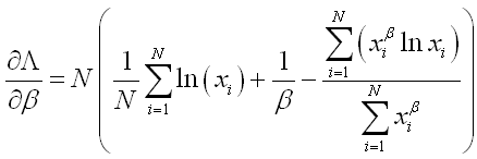
Replacing η using its MLE solution in Eqn. (3) and taking the derivative with respect to β, we get:

(5)

It can be proved that there is a unique solution for β to make Eqn. (5) equal to 0. The detail of the proof is not given in this article.

Case 3: The Shape Parameter β Is Given

If β < 1, it is clear that there is no MLE solution for γ in Eqn. (2),  The likelihood value goes to positive infinity as γ → tmin.

If β = 1, Eqn. (2) becomes:

(6)

The derivative with respect to γ is:

The likelihood value increases with γ. So the MLE solution for γ is γ = tmin.

When 1 < β < 2, we know from the published papers [1, 2] that the MLE estimators for γ exist in general, but are not asymptotically normal.

When β≥ 2, the MLE solution always exists and the information matrix is asymptotically normal [1, 2].

The Confidence Bounds for γ

When the MLE method is used, one commonly used method for calculating the confidence bounds for the parameters is the Fisher information matrix method. The estimated Fisher information matrix is defined as:

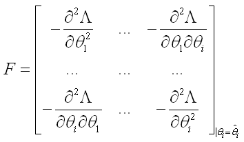
This is the 2nd order derivative of the log-likelihood function with respect to each parameter at the MLE solution.

The variance and covariance matrix of the parameters is:

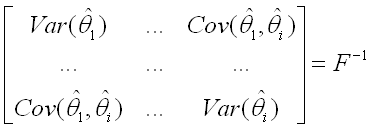
If we assume the MLE solutions are asymptotically normally distributed, then the confidence bounds of the parameters are:

(7)

For more detailed discussion, please refer to https://help.reliasoft.com/reference/life_data_analysis/lda/confidence_bounds.html.

Because variance must be a positive value, the 2nd order derivative in the Fisher information matrix for each parameter at the MLE solution must be negative. Otherwise, no variance can be estimated.

Let’s use a simple 2-parameter Weibull example to explain this. Assume we have the following failure times: 15, 34, 56, 67, 118 and 234. The MLE solutions are:

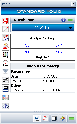
The 3D plot for the likelihood values is shown next.

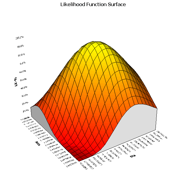
The x-axis and y-axis are the two parameters β and η. The z-axis is the normalized log-likelihood value. The MLE solution for β and η are the values corresponding to the peak of the plot. At the peak, the 1st order derivative of each parameter is 0. The 2nd order derivative of each parameter is negative, because the 1st order derivative changes from positive to negative.

However, for the 3-parameter Weibull distribution, we have the three cases discussed above. For Case 1, where we need to estimate all three parameters, there is no global MLE solution for γ (no global peak in the likelihood value vs. γ plot), so no confidence bounds can be obtained for γ using the Fisher information matrix. For Case 2, γ is given, so there are no confidence bounds for γ. For Case 3, where β is given and is greater than 2, there is a MLE solution for γ, and the confidence bounds can be obtained from the Fisher information matrix. Otherwise, no bounds exist for γ, either because there is no MLE solution for γ (when β < 1) or because the solution for γ is tmin (when β = 1).

A Hybrid Method to Estimate Parameters for the 3-Parameter Weibull Distribution

In Weibull++, we provide a hybrid method for parameter estimation for the 3-parameter Weibull distribution. By default, the least squares estimator (rank regression method) of γ is used, and is treated as fixed.  Once γ is fixed, this becomes Case 2 discussed previously, and the MLE estimators for β and η can be estimated correctly. This is controlled by the Use true 3-P MLE on Weibull check box on the Calculations page of the Application Setup, which is cleared by default.

For example, consider the following data set: 100, 218, 334, 556, 867 and 1234.

When Use true 3-P MLE on Weibull is not selected, the calculated results are:

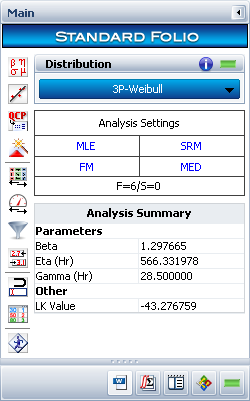
γ is 28.5, which is calculated using the least squares estimation method.

The 3D likelihood value plot is shown next.

 

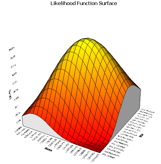
This plot shows that there are MLE solutions for β and η. The probability plot is shown next.

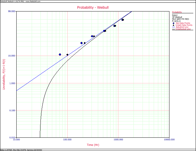
This plot shows that the estimated probability line fits the data points very well.

When Use true 3-P MLE on Weibull is selected, the calculated results are:

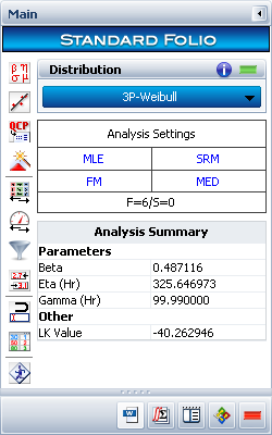
Since there is no true MLE when γ is not given, the returned γ is 99% of the smallest failure time. The MLE β and η are estimated as if the γ is fixed. (Note that in the latest version of Weibull++, γ = 99.99% of the smallest failure time, due to changes in the software.)  The 3D likelihood value plot is:

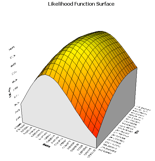
This plot shows that there are MLE solutions for β and η since γ is treated as fixed. The probability plot is shown next.

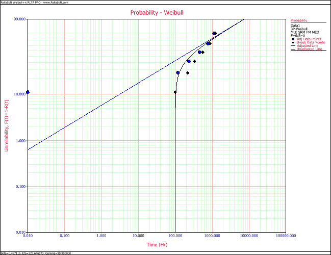
This plot shows that the estimated probability line does not fit the data points very well.

From this example, we can see that the best way of estimating the 3-parameter Weibull distribution using MLE is to use the least squares estimator of γ, and then calculate the MLE solution for β and η by treating γ as fixed.

Conclusion

In this article, we briefly discussed the MLE solution for the 3-parameter Weibull distribution. For a given data set from life testing, usually no information is available on the three parameters. All of the parameters have to be estimated, and users need to choose how to estimate them. We recommend using the hybrid method provided in Weibull++ in order to avoid the problems inherent in MLE parameter estimation with three unknown parameters. For more discussion on parameter estimation, please refer to http://reliawiki.org/index.php/Parameter_Estimation.

References

[1] R. L. Smith, “Maximum Likelihood Estimation in a Class of Non-regular Cases,” Biometrika, vol. 72, no. 1, pp. 67-90.
[2] H. Hirose, “Maximum Likelihood Estimation in the 3-parameter Weibull Distribution: A look through the Generalized Extreme-value Distribution,” IEEE Transaction on Dielectrics and Electrical Insulation, vol.3, no.1, pp. 43-55.