Unbiasing Beta for the Crow-AMSAA (NHPP) Model

[Editor's Note: This article has been updated since its original publication to reflect a more recent version of the software interface.]

The Crow-AMSAA (NHPP) model is probably the most popular model in reliability growth and repairable system analysis. With this model, maximum likelihood estimation (MLE) is used to estimate the parameters. However, it is well known that the MLE solution for the shape parameter in any model is biased (i.e., the estimated beta value is too high), which affects the accuracy of the results. This is a particular concern when working with small sample sizes. This article will demonstrate how the bias is corrected for Crow-AMSAA in RGA. This is also applicable to the Crow Extended, Crow Extended - Continuous Evaluation and power law models.

Crow-AMSAA (NHPP) Model

The instantaneous failure intensity of a system is a power function in the Crow-AMSAA model. It is:

(1)

where λ and β are the two model parameters. Sometimes this model is also called the power law NHPP model. The function for the expected number of failures is:

(2)

The Crow-AMSAA model can be used for both time and failure terminated data. For example, if a test ends at 300 hours even though the last failure was at 286.1 hours, then it is a time terminated test. If the test ended at the time of the last failure (i.e., 286.1 hours), then it is a failure terminated test.

The data in the next table are from a time terminated test. The F events are failures, and the End event is the end of the test.

Table 1: Data from a time terminated test

 

The following data are from a failure terminated test. In this case, the last failure time is the treated as the end of the test.

Table 2: Data from a failure terminated test

 

In order to use MLE, we need to get the likelihood function for a set of data. The probability density function (pdf) of the ith failure given that the (i-1)th failure occurred at ti-1 is:

(3)

For failure terminated data, the likelihood function is the product of the pdf of each failure. It is:

(4)

where n is the total number of failures.

For time terminated data, the system is working from the last failure time to the test end time T. Therefore, the following conditional reliability equation is used to model the likelihood that no failure occurs by time T.

(5)

Multiplying Eqn. (5) with the pdf of each failure, we get the likelihood function:

(6)

Let T* be either T (time terminated) or tn(failure terminated). Eqns. (4) and (6) can be written as:

(7)

Taking the natural log on both sides:

(8)

Differentiate Eqn. (8) with respect to:

(9)

Set the above equation equal to zero and solve for β to get the MLE solution:

(10)

Bias Correction

ln(T*/ti)β, i= 1,…, n are ordered statistics from an exponential distribution with a parameter of 1. This can be explained from the simulation point of view.

The reliability function for an exponential distribution with a parameter of 1 is Pi= exp(-xi). For time terminated data, it can be seen that Pi is a number between 0 and 1. So xi (i = 1,…,n ) is a random number from an exponential distribution with a parameter of 1.

For failure terminated data, xn can be removed and i ranges from 1 to n - 1. This is because:

The sum of k random exponential variables with a parameter of 1 is a Gamma random variable with parameters of k and 1. Therefore, for failure terminated data:

(11)

One variable is eliminated because ln(tn/tn) = 0, so there are only n - 1 random variables in the sum in Eqn. (11). Since Y follows a gamma distribution Gamma(n - 1, 1), 1/Y is an inverse gamma distribution, 1/Y ~InverseGamma(n - 1, 1). The expected value of 1/Y is:

(12)

From Eqn. (10), we know:

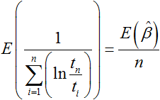
Therefore:

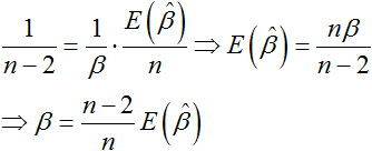
(13)

Eqn. (13) shows is biased because its expected value is not β. Therefore, the factor (n - 2)/n is used to remove the bias.

For time terminated data, since:

(14)

We can also get:

(15)

Example:

The Calculate unbiased beta check box on the Calculations page of the Application Setup (File > Application Setup) is used to select whether the software will correct the bias, when applicable.

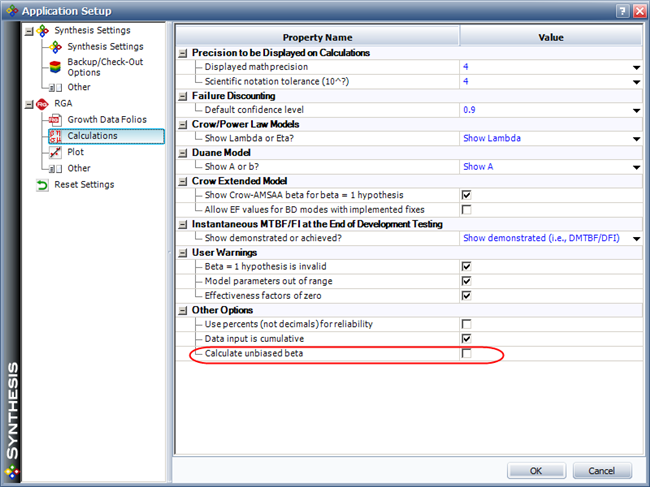
If this option is cleared when you calculate the time terminated data in Table 1, the (biased) MLE beta value will be calculated, as shown next in the Results area.

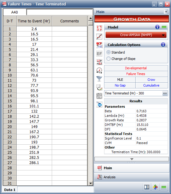
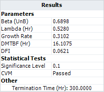
For an MLE beta of 0.7163 and with 27 data points (n = 27), we can calculate the unbiased beta as follows:

If you select the Calculate unbiased beta option and recalculate the folio. The unbiased value will appear, as shown next and indicated with the "Beta (UnB)" label:

Conclusion

In this article, we explained why the MLE betaof the Crow-AMSAA model is biased and how to correct it. When the sample size is large, there may be only a small difference between the biased and unbiased beta, as illustrated in the example. When the sample size is small (e.g., less than 5), the difference is relatively large, so the unbiased beta is preferred.