Demonstrating a Difference in Life Using the Difference Detection Matrix
In the manufacturing industry, design/test engineers often need to design demonstration tests for devices and materials from different suppliers. To do this, they need to decide which sample size and testing time are most appropriate for the test. The Synthesis version of Weibull++ has a new tool, the Difference Detection Matrix, which can help engineers make such decisions. The Difference Detection Matrix calculates how much test time is required before it is possible to detect a statistically significant difference in the mean life or BX% life (e.g., B10 life) of two product designs by analyzing the data from a reliability life test. The engineer can use this tool to evaluate different test plans in order to choose the most efficient way to compare the reliability metric of two designs.
In this article, we will use an example to illustrate how to use this new tool. If you have Synthesis installed on your computer, you can download and view the example file (5.25 MB, *.rsrp) here.
Example
A test engineer was asked to evaluate water pumps from two different manufacturers. Manufacturer A claims that its pump’s (Type A) failure time follows a Weibull distribution with beta = 2 and a mean life of 600 hours. Manufacturer B claims that its pump's (Type B) failure time follows a lognormal distribution with log-std = 0.8 and a mean life of 1,050 hours. The engineer was assigned the task of demonstrating a mean life difference between these two products. The budget allocated to the task is $9,000. One pump A device costs $100, and one pump B costs $120. One hour of test time costs $2.
The engineer used Weibull++ to do the analysis. To create a new Difference Detection Matrix, he chose Insert > Tools > Test Design, and in the Test Design Assistant (shown in Figure 1), he chose Difference Detection Matrix.
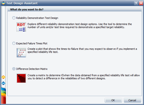
Figure 1 - Test Design Assistant
In the new Matrix, he specified that he will be comparing the mean life of each design with a confidence level of 90%. Then he provided the inputs shown in Figure 2.
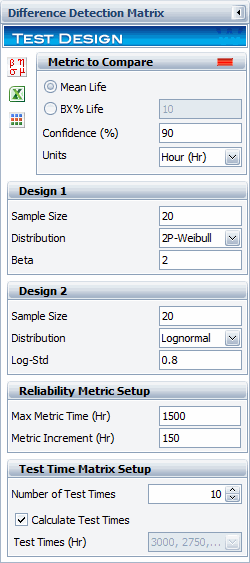
Figure 2 - Inputs to the Matrix control panel
As these inputs show, the engineer decided to first try a sample size of 20 for both products, and he specified that the tool will consider all mean life values up to 1,500 hours (Max Metric Time) in increments of 150 hours (Metric Increment).
Next, in the Test Time Matrix Setup area, he selected to evaluate 10 different test times. After clearing the Calculate Test Times check box, he clicked inside the Test Times field to enter the test times in the table shown in Figure 3.
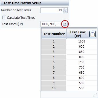
Figure 3 - Specifying test times to evaluate
The resulting Matrix is shown in Figure 4.
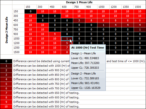
Figure 4 - Difference Detection Matrix
The columns represent the possible mean life values for Design 1 (here, Design A), and the rows represent possible mean life values for Design 2 (here, Design B). The number inside each cell indicates what test time within the specified range (if any) would be sufficient to detect a difference in the specified reliability metric. Since Design A has an expected life of 600 hours and Design B has an expected life of 1,050 hours, the engineer needed to click the cell at the fourth column and seventh row. The estimated mean life and its confidence interval for each design and at 1,000 hours of test time are displayed next to the cursor in Figure 4. Since the two confidence intervals do not overlap, the engineer knew that a difference in mean life could be detected with 1,000 hours of test time.
The test engineer wanted to use the shortest test time possible within the provided budget. So he gradually increased the test samples to 45 (in increments of 5) and recalculated the matrix each time. The sample sizes, corresponding test times and associated costs (calculated by combining the costs of test units and testing time as described above) are shown in Table 1. Since the budget is limited to $9,000, the engineer decided to pick the plan with a sample size of 35.
Table 1 - Different Test Plans with Different Sample Sizes
| Sample Size for A | Sample Size for B | Test Time (Hr) | Cost ($) |
| 20 | 20 | 1,000 | 6,400 |
| 25 | 25 | 650 | 6,800 |
| 35 | 35 | 600 | 8,900 |
| 40 | 40 | 600 | 10,000 |
| 45 | 45 | 500 | 10,900 |
With the current mean life values, the engineer wanted to see the expected failure times for these two products. So he opened the Test Design Assistant window again and chose Expected Failure Time Plot. In the control panel, he entered the expected failure model for Design A. For Design A with the Weibull distribution, if the mean life = 600 and beta = 2, then eta can be solved by:

|
(1) |
For Design B with the lognormal distribution, if the mean life = 1,050 and log-std = 0.8, then the mean of the logarithms of the failure times could be solved by:
|
|
(2) |
So the expected failure model for Design A is a Weibull distribution with beta = 2 and eta = 677. And the failure model for Design B is a lognormal distribution with log-mean = 6.64 and log-std = 0.8. 35 units would be used for testing, and two-sided 90% confidence bounds would be chosen. The expected failure times for Design A are plotted in Fig. 5.
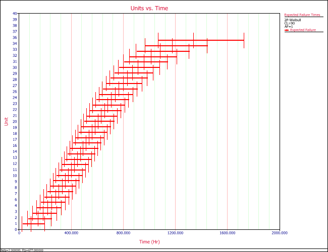
Figure 5 - Expected Failure Time Plot for Design A
The expected failure times for Design B are plotted in Fig 6.
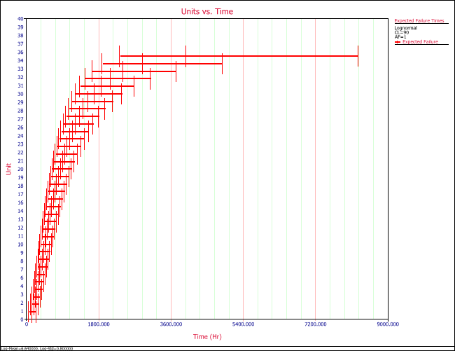
Figure 6 - Expected Failure Time Plot for Design B
With the planned test time and these expected failure times in mind, the engineer began the test.
Conclusion
In this article, we used an example to illustrate how to use the Difference Detection Matrix to design a test intended to demonstrate a difference in life between two products. (For simple cases like this example, the Difference Detection Matrix can be used—but for more complex cases, advanced design of experiments (DOE) techniques may be more appropriate.) The Matrix can help a design/test engineer choose a sample size and testing time, with the goal of adopting an economically optimized test plan.