A Response Surface Approach for Robust Parameter Design

[Editor's Note: This article has been updated since its original publication to reflect a more recent version of the software interface.]

Robust parameter designs have been used widely in industry. In Issue 122 of the Reliability Hotwire, we discussed using Taguchi’s method to design robust products and processes. An example with a cross-array design using ReliaSoft’s DOE++ was given. In this article, we will use a single-array design with a response surface method approach for robust parameter design.

The Secret of Robust Parameter Design

The following diagram illustrates the relation between input variables and output response for a system. The system could be either a product or a process.

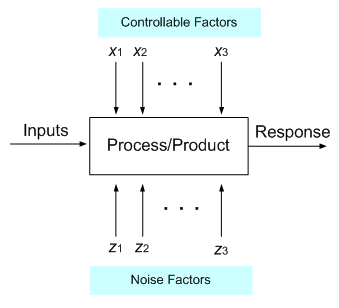
Figure 1 - System diagram

There are two types of factors in the above figure: control factors and noise factors. Control factors are variables that can be controlled, such as design parameters or process variables. Noise factors are variables that are very difficult to control, such as ambient temperature and humidity. Both types of factors will affect the response. For example, consider a system where, when the input variable is 5 volts, the system’s response is 10 mA at a room temperature of 20°C. However, when the room temperature is 30°C, the system response is 13 mA with the same input of 5 volts. This system is not robust to room temperature, although ideally it should be. Therefore, we need to adjust the control factors to make the system robust. 

The secret of robust design is understanding the control and noise factor interactions. The following plot illustrates this point.

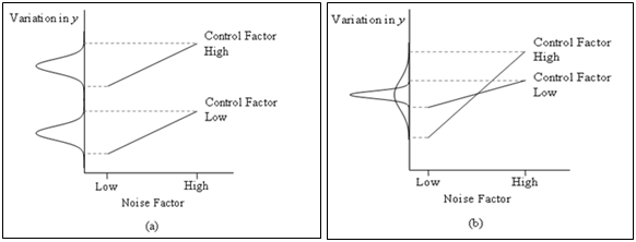
Figure 2 - Control and noise factor interaction

There is one noise factor and one control factor in Figure 2. The value of the noise factor can change from low (-1) to high (+1). The change of this noise factor causes variation of response y.

In Figure 2(a), no matter what level the control factor is, the amount of change for y is the same. Therefore, it is impossible to adjust the level of the control factor to reduce the effect of the noise factor.

In Figure 2(b), when the control factor is at its low level, the change of y is much smaller than that when the control factor is at its high level. Therefore, setting the value of the control factor at its low level will reduce the effect of the noise factor, or in other words, will make the system robust to the noise factor.

In summary, Figure 2(a) shows a situation where there is no interaction between the control and the noise factor, while Figure 2(b) shows a situation where they do have interaction. Because of this interaction, it is possible to have robust design for the system.

The Single Array Method for Robust Design

Let x be the control factor and z be the noise factor. The relationship between them and the response y is: [1]

(1)

The variation of the noise factor z will be transformed to y. As discussed above, if x and z have interactions, then the variation in y can also be reduced by changing the settings of x. For example, consider a simple model such as:

(2)

Eqn. (2) has two control factors, x₁ and x₂, and one noise factor, z. ε is the error term, following a normal distribution with mean of 0 and standard deviation of Var(ε). Assume Eqn. (2) is in terms of the coded values of each variable and z follows a normal distribution with mean of 0 and standard deviation of Var(z). Then, the expected value and variance of y are:

(3)

We can adjust x1 to bring y to its target value and adjust x2 to reduce the variance of y. Eqn. (3) clearly shows the importance of the control-by-noise interaction in reducing the variation in y.

Example: The Pilot Plant Experiment

A single-replicate factorial experiment is conducted to study the factors affecting the filtration rate of a chemical product. The four factors are: temperature (A), pressure (B), concentration of formaldehyde (C) and stirring rate (D). Factor A is treated as noise, since it is hard to control. Each factor has two levels. The engineer wants to maintain the filtration rate at 75 gallons per hour and reduce its variation. The design and results are given below. [2]

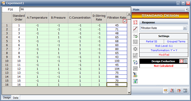
Figure 3 - Design matrix and response

The initial model is shown next.

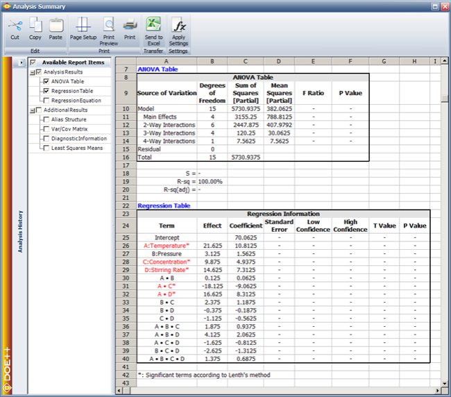
Figure 4 - Results of the initial model

The results show that factors A, C and D are significant, as are the interactions of AC and AD. The engineer pools the non-significant effects into error by excluding those effects from the model, as shown next.

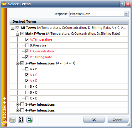
The recalculated final model is:

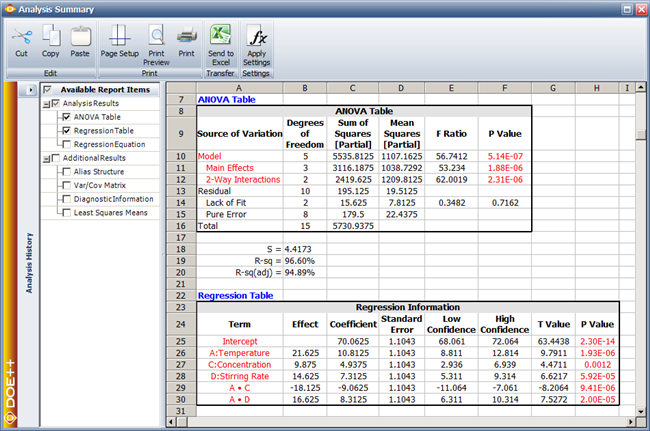
Figure 5 - Results of the final model

Therefore, the final equation for response y is:

(4)

where z is the noise factor A (temperature), x2 is factor C (concentration) and x3 is factor D (stirring rate). Using Eqn. (3), the expected value of y and its variance are:

(5)

In Figure 5, S (located below the ANOVA table) is the estimated standard deviation. Its square is the estimated variance (i.e., Var(ε) = 4.41732 = 19.5125). Therefore, the problem in this experiment becomes an optimization problem:

(6)

Using the solver in Micrososft Excel®, the optimal values for x2 and x3are 0.8861 and 0, respectively. At these settings, the estimated variance of y is 22.29498.

In this example, the engineer wanted to maintain the filtration rate at 75 gallons per hour. If the engineer wanted to maximize the filtration rate and at the same time to reduce the variance, the multiple response optimization method explained in the Experiment Design and Analysis reference book could be used (https://help.reliasoft.com/reference/experiment_design_and_analysis/doe/response_surface_methods_for_optimization.html#MultipleResponses).

Conclusion

In this article, a single array and a response surface modeling method are used for robust parameter design. This is an alternative to the traditional cross-array robust design method. The optimization method in this article can be used when the objective is to maintain the response at a given value and reduce its variation. Otherwise, the location and dispersion modeling strategy should be used with either a cross-array or a single-array design. For more detail, please refer to the Reliability Hotwire articles on variability analysis in DOE++ and on robust parameter design.

References

[1] C. F. Wu and M. S. Hamada, Experiments: Planning, Analysis, and Optimization, 2nd ed. New York, NY: John Wiley & Sons, Inc., 2009, pp. 518-520.
[2] R. H. Myers and D. C. Montgomery, Response Surface Methodology, 2nd ed. New York, NY: John Wiley & Sons, Inc., pp. 557-560.