Taguchi Orthogonal Array Designs
Taguchi Orthogonal Array (OA) design is a type of general fractional factorial design. It is a highly fractional orthogonal design that is based on a design matrix proposed by Dr. Genichi Taguchi and allows you to consider a selected subset of combinations of multiple factors at multiple levels. Taguchi Orthogonal arrays are balanced to ensure that all levels of all factors are considered equally. For this reason, the factors can be evaluated independently of each other despite the fractionality of the design. This article will show how to perform a Taguchi OA design using DOE++.
In the Taguchi OA design, only the main effects and two-factor interactions are considered, and higher-order interactions are assumed to be nonexistent. In addition, designers are asked to identify (based on their knowledge of the subject matter) which interactions might be significant before conducting the design.
Consider an example where a truck front fender’s injection-molded polyurethane bumpers suffer from too much porosity [1]. A team of engineers conducted a Taguchi OA design to study the effects of several factors related to the porosity.
Table 1: Factors
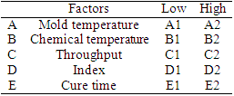
The team also decided to consider interactions AB and BC. They took two measurements of porosity (for porosity values, smaller is better). They also decided to use the L8 orthogonal array for this design. Table 2 shows the alias relation for L8 arrays.
Table 2: L8 (2^7) Arrays

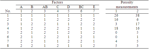
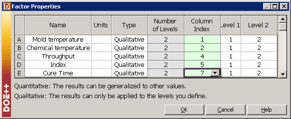
In Table 2, column 3 is the alias of the interaction of column 1 and column 2 (in red), while column 6 is the alias of the interaction of column 2 and column 4 (in red). Since interactions AB and BC are considered significant in this example, the main factors A, B, C, D and E are assigned to columns 1, 2, 4, 5 and 7. The interaction factors AB and BC are assigned to columns 3 and 6.
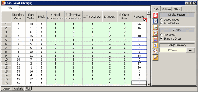
Table 3 shows the L8 orthogonal array and the porosity measurements the team took.
Table 3: L8 Orthogonal Array
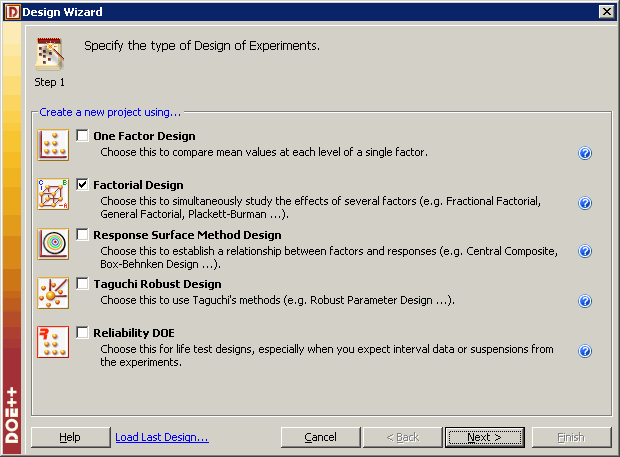
To use DOE++ to perform the Taguchi OA design, add a folio to a project by choosing Project > Add Standard Folio. In Step 1 of the Design Wizard, select the Factorial Design option because Taguchi OA design actually is a factorial design.
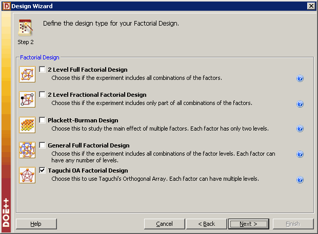
In Step 2 of the Design Wizard, choose the Taguchi OA Factorial Design option.
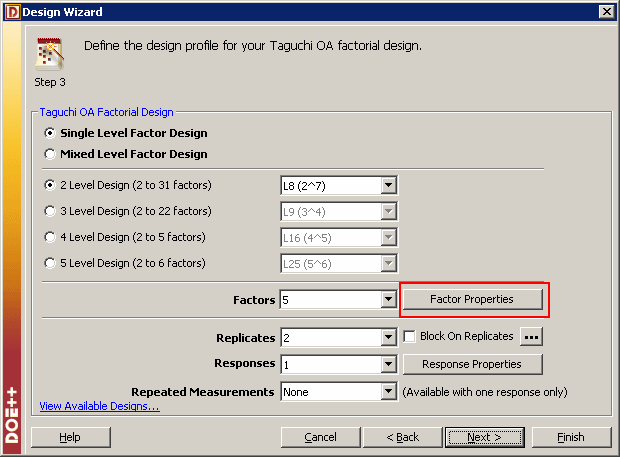
In Step 3 of the Design Wizard, select the 2 Level Design option with a L8 (2^7) array and specify that there are five factors with two replicates and one response.
Click Factor Properties and assign the factors as shown next:
After creating the design folio and entering the data from Table 3, the DOE++ folio will look like this:
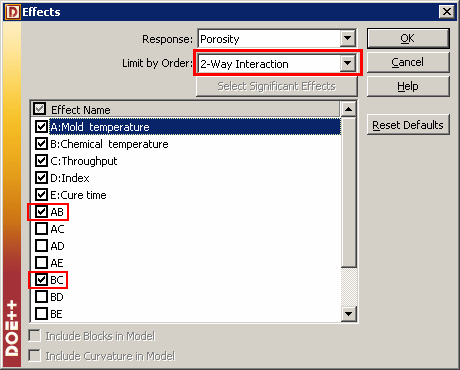
The interactions are not currently included in the reduced L8 array. In order to take them into account, they need to be included as a 2-Way Interaction using the Effects window (Data > Select Effects).
Click the Calculate icon to analyze the experimental data. On the Analysis tab, the ANOVA table and the Regression Information table should look like this. The factors in red means they are significant.
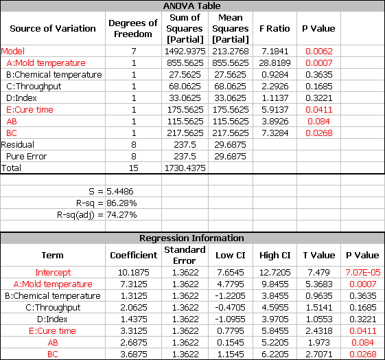
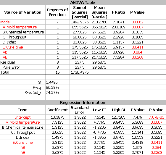
From the ANOVA table above, it is interesting to see that the interaction BC is significant while both main factors B and C are not significant. According to the Effect Heredity Principle [2]: "In order for an interaction to be significant, at least one of its parent factors should be significant." There is something hidden here. Look back to Table 2 again. Column 6 is not only the alias of column 2 and column 4 (in red, which is the interaction BC in this example); it is also the alias of column 1 and column 7 (in green, which is the interaction AE in this example). Factors B and C are not significant, thus their interaction BC should not be significant either. There is a great chance that it is the interaction AE which is significant, not BC. This is a Resolution III design, where the interaction BC and AE are confounded with each other. So the next step is to replace interaction BC by interaction AE in the model and run the analysis again.
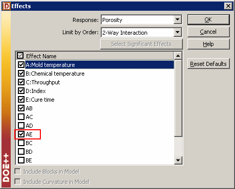
The ANOVA table for the new analysis is shown below. It is identical to the previous result, which confirms that the significant interaction is AE not BC.
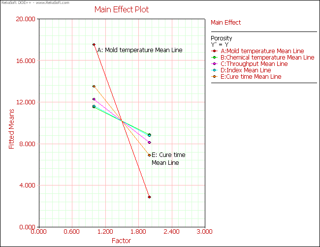
The Main Effects plot is shown next. The plot shows that factors A and E are significant while the other three factors are not, which is the same as the results shown in the ANOVA table.
The ANOVA table shows that factors B, C and D are not significant. However, interactions AB and AE are significant. Thus in the reduced model, factor B cannot be removed; the factors that can be removed are C and D. In the Effects window, remove factor C and D and do the analysis again.
The new ANOVA table and Regression Information table are shown below.
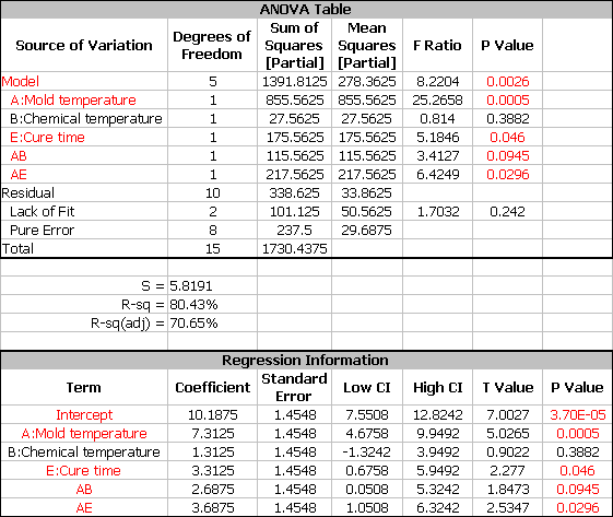
To identify which factor settings can provide the best design, open the Diagnostics Window by choosing Data > Diagnostics. The "Fitted Value (YF)" column shows the expected porosity for the factor settings under different runs.
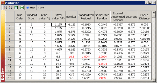
The table shows that run order 4 (standard order 14) and run order 9 (standard order 6) give the best result. The predicted porosity is 1.125. Note that because the experiment used two replicates, run order 9 and run order 4 used the same settings: mold temperature high, chemical temperature low, throughput high and cure time low.
Conclusions
This article described the Taguchi orthogonal array design and provided an example using DOE++ that showed how to use the design to create an experiment and analyze the data.
References
[1] Kai Yang and Basem El-Haik. "Taguchi's Orthogonal Array Experiment," in Design for Six Sigma: A Roadmap for Product Development, McGraw-Hill, 2008, pp. 469-497.
[2] C. F. Jeff Wu and Michael Hamad, "Full Factorial Experiments at Two Levels," in Experiments: Planning, Analysis, and Parameter Design Optimization, John Wiley & Sons, Inc. 2000, p. 112.