Determining the Sample Size for a Life Test Based on the Shape Parameter of the Weibull Distribution
[Editor's Note: This article has been updated since its original publication to reflect a more recent version of the software interface.]
The Weibull distribution is one of the most important distributions in life data analysis. The value of its shape parameter (beta) influences the failure rate behavior; therefore, reliability engineers are often interested in designing life tests that can accurately estimate the value of beta. In this article, we will use SimuMatic®, a simulation tool in Weibull++, to study the property of the shape parameter when estimated using the maximum likelihood estimation (MLE) method. Based on the results of the simulation study, we will provide simple rules on how to determine the appropriate sample size for a life test according to an accuracy requirement for beta.
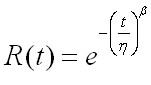
To illustrate how SimuMatic generates data, consider the reliability function for the Weibull distribution:
|
(1) |
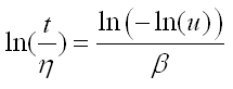
where β is the shape parameter and η is the scale parameter. In order to generate a random failure time t, a random number u from a uniform distribution U(0, 1) is generated first and then used to represent the reliability value R(t). The failure time t is then obtained by using the following equation:
|
(2) |
From Eqns. (1) and (2), we can see that the value of η affects the generated failure times proportionally, but it doesn’t have an effect on the values for β. This is illustrated in the following example.
Example 1
-
In SimuMatic, generate a data set for a 2-parameter Weibull distribution with Beta = 2 and Eta = 100, as shown next.
-
On the Censoring tab, select No Censoring.
-
On the Settings tab, set the number of data sets to 5 and the number of points to 30.
-
On the Analysis tab, select Maximum Likelihood (MLE). Leave all other settings at default.
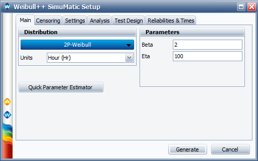
Click Generate to start the simulation. The following table shows the estimated beta and eta values for each data set, when estimated using MLE:
| Data Set | Beta | Eta |
| 1 | 1.8101 | 103.8684 |
| 2 | 2.2792 | 89.8633 |
| 3 | 2.3836 | 99.6618 |
| 4 | 2.3017 | 132.6608 |
| 5 | 2.8522 | 101.3464 |
-
If we change the input value of eta from 100 to 1, while keeping the rest of the settings unchanged, the estimated beta and eta values for each data set would be:
| Data Set | Beta | Eta |
| 1 | 1.81 | 1.0387 |
| 2 | 2.2792 | 0.8986 |
| 3 | 2.3836 | 0.9966 |
| 4 | 2.3017 | 1.3266 |
| 5 | 2.8522 | 1.0135 |
From Tables 1 and 2, we can see that the input value of eta has no effect on the estimated beta values. No matter what the value of eta is, the estimated beta values will remain the same. Therefore, the scale parameter does not affect the shape parameter of the Weibull distribution. But how does sample size affect the shape parameter?
In SimuMatic, we could use beta values of 0.5, 1, 1.5, 2 and 2.5, together with sample sizes (number of points) of 5, 10, 20, 50 and 100. For each combination of beta value and sample size, we generate 1,000 data sets and obtain an estimate of the beta. Next, we obtain the mean and standard deviation of the beta values. These values are given in Tables 3 and 4, as shown next.
| Mean | Sample Size | |||||
| 5 | 10 | 20 | 50 | 100 | ||
| Beta | 0.5 | 0.7140 | 0.5836 | 0.5381 | 0.5166 | 0.5112 |
| 1 | 1.4219 | 1.1598 | 1.0678 | 1.0241 | 1.0145 | |
| 1.5 | 2.1329 | 1.7509 | 1.6142 | 1.5497 | 1.5217 | |
| 2 | 2.8558 | 2.3346 | 2.1522 | 2.0663 | 2.0448 | |
| 2.5 | 3.5698 | 2.9182 | 2.6903 | 2.5828 | 2.5560 | |
| Standard Deviation |
Sample Size | |||||
| 5 | 10 | 20 | 50 | 100 | ||
| Beta | 0.5 | 0.4032 | 0.1825 | 0.1034 | 0.0566 | 0.0403 |
| 1 | 0.8064 | 0.3662 | 0.2069 | 0.1131 | 0.0807 | |
| 1.5 | 1.2096 | 0.5494 | 0.3103 | 0.1697 | 0.1210 | |
| 2 | 1.6129 | 0.7325 | 0.4138 | 0.2262 | 0.1613 | |
| 2.5 | 2.0135 | 0.9156 | 0.5172 | 0.2828 | 0.2017 | |
From Tables 3 and 4, we can see that the values for the mean and the standard deviation have the same proportions as the beta values that were used in the simulation. For example, in Table 3, the mean value for beta = 1 is twice the mean value for beta = 0.5. This is also the case for the standard deviation values.
The following ratio represents the relative uncertainty of the estimated beta:

|
(3) |
where the denominator represents the MLE solution of beta and the numerator is the standard deviation value of beta. This ratio is usually called the coefficient of variation (CV). From the results of the simulation test, we know that the ratio is constant for all the beta values for a given sample size and that it is independent of the value of beta. Therefore, Eqn. (3) can be used to design a life test without having to guess the value of beta in the Weibull distribution.
Rule 1: Determine the Sample Size for a Life Test Based on the Bias Requirement of Beta
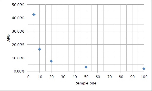
From Table 3, we can see that the bias of the estimated beta decreases as the sample size increases. In this case, bias is the difference between the value of beta that was used as input for the simulation and the value of beta that was estimated from the simulation. From Table 3, we can also see that the relative bias is a function of sample size and it is independent of the values of beta and eta. The average relative biases calculated from all the simulation runs for the different sample sizes are summarized in the following table.
| Sample Size (n) | 5 | 10 | 20 | 50 | 100 |
| Average Relative Bias (ARB) | 42.55% | 16.58% | 7.45% | 3.13% | 1.92% |
The relative bias (RB) of each combination is calculated using:

|
(4) |
The following plot shows the data in Table 5.
If we fit the data in Table 5 to a power function, then we have:

|
(5) |
If the expected ARB is required to be less than 20%, then Eqn. (5) tells us that the number of samples n to be used in a life test needs to be greater than 9. Therefore, Eqn. (5) can be used to determine the sample size of a life test based on the required bias of beta.
Rule 2: Determine the Sample Size for a Life Test Based on the Ratio of the Upper and Lower Bound of the Estimated Beta
The ratio of the bounds represents how wide the confidence bounds are. For a given confidence level, the bigger the ratio, the larger the uncertainty of the estimation.
The 1-sided upper and lower bounds of beta, when estimated using MLE, can be obtained by:
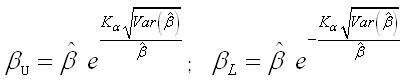
|
(6) |
where  is the 1- ∝ percentile of the standard normal distribution. The ratio of βU and βL is:
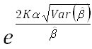
|
(7) |
This ratio is usually used to represent the uncertainty of the estimate of beta. The larger the sample size, the smaller the bounds ratio. Because the ratio is affected only by the sample size, and not by the values of beta and eta, it follows that Rule 2 can also be used to plan a life test without having to guess the values eta and beta for the Weibull distribution.
From Tables 3 and 4, we can calculate the average coefficient of variation (ACV) for different sample sizes, as shown in the next table.
| Sample Size (n) | 5 | 10 | 20 | 50 | 100 |
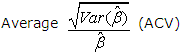
|
0.5656 | 0.3139 | 0.1926 | 0.1097 | 0.0792 |
The following plot shows the data from Table 6.

If we fit the data in Table 6 to a power function, then we have:

|
(8) |
For a 90% 1-sided confidence bound, the ratio of βL and βU is:
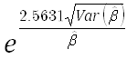
|
(9) |
If the expected bounds ratio is required to be less than 1.5, then Eqn. (9) tells us that the value of the ACV needs to be less than 0.1582. Therefore, if we set the ACV to 0.1582 in Eqn. (8), the minimum sample size n is estimated to be 30.59 or 31. The next example validates Rule 2 using SimuMatic. A similar validation can be done for Rule 1.
Example 2
-
Assume the bounds ratio is required to be less than 1.5. From the study of Rule 2, we know that the minimum sample size is 31. In SimuMatic, create a new simulation using the following settings:
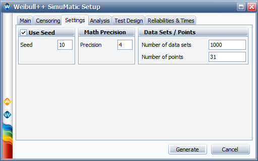
Make sure that the number of points is 31, which is the minimum sample size. Set the number of data sets to 1,000. For the 2P-Weibull parameters, we can use any values for beta and eta because Rules 1 and 2 are not dependent on those values. This is the beauty of these two rules. For this example, use Beta = 2.3 and Eta = 1.
-
On the Censoring tab, select No Censoring.
-
On the Analysis tab, select Maximum Likelihood (MLE). Leave all other settings at default. Click Generate to start the simulation.
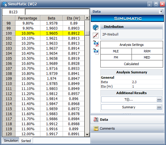
In the results, view the “Sorted” data sheet. The following figure shows the 90% 1-sided lower confidence bound of beta.
Shown next is the 90% 1-sided upper confidence bound of beta:
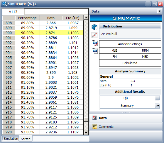
The ratio of βU and βL is 2.8741/1.9605 = 1.4660, which is indeed less than the required value of 1.5.
Conclusion
In this article, two simple rules are proposed for determining the sample size of a life test where all samples are tested to failure. Eqns. (5) and (8) were created based on the simulation results of SimuMatic. Although they are not from a rigid mathematic derivative, examples show that they are accurate and simple to apply. Rule 2, however, is more commonly used than Rule 1 because bias is usually not a big concern compared to the uncertainty in the beta estimates. For more details on MLE and confidence bounds, please refer to [1, 2].
References
[1] Meeker, W. and Escobar, L, Statistical Methods for Reliability Data, John Wiley & Sons, Inc, New York, 1998.
[2] Nelson, W., Applied Life Data Analysis, John Wiley & Sons, Inc., New York, 1982.