Using the Cumulative Binomial Equation for Reliability Demonstration Test Design and for Estimating the Parameters of a Data Set with Zero Failures
[Editor's Note: This article has been updated since its original publication to reflect a more recent version of the software interface.]
In this article, we will introduce the cumulative binomial equation and explore two potential applications for reliability engineering. First, we will explain how the equation can be applied for designing a Reliability Demonstration Test (RDT) that will be effective for demonstrating that a certain product has met or exceeded a given reliability at a given confidence interval. For this application, the equation can be adapted to apply to a situation in which no failures are expected to occur in the test. Next, we will discuss how that special case of the equation can also be applied for estimating the unknown parameter in a data set that does not contain any failures.
Reliability Demonstration Test Design
One of the most commonly used methods for RDT design is based on the following binomial equation:
where n is the sample size and r is the number of failures allowed during the test.
In Eqn. (1), we assume that the test is either for a one-shot system (e.g., a missile that is only classified as being successful or failed whenever launched) or for a situation where the test duration is the same as the time when the required reliability is evaluated. If the test duration is different from the time when the reliability is evaluated (e.g., the test duration is 200 hours while the required reliability is evaluated at 500 hours), a distribution for the failure time has to be provided. Distributions commonly used to describe the failure time include the Weibull, lognormal and exponential distributions.
For example, suppose that the goal is to demonstrate that the reliability at time t meets the required reliability RL(t) at a specified confidence level, CL. For a test duration T0, where T0 ≠ t, we will need to convert the required reliability at time t to the reliability at the test duration T0. For a Weibull distribution, its reliability function is:
where β is the shape parameter and η is the scale parameter. The conversion procedure is given next.
Step 1: Use the requirement on the reliability at time t in Eqn. (2) and express the equation in terms of the scale parameter ηL by:
Step 2: Next, use ηL to calculate the requirement on the reliability at test time T0:
Once RL(T0) is obtained, Eqn. (1) can be used directly. Note that if β is given, this conversion can indirectly demonstrate the required RL(t).
Now, suppose that there are zero failures in the test, r = 0. The test becomes the so-called "zero-failure test" or "success test." Accordingly, Eqn. (1) becomes:
where ηL is the lower bound of η. Taking the logarithm of both sides of Eqn. (3) yields:
It is well known that the CL (left side tail) percentile of a X2 distribution with two degrees of freedom is:
As a result:
One can see that the random variable ![]() follows a X2 distribution with two degrees of freedom. Therefore, if the values
of β, the required RL(t)
and the time t are given, Eqn. (4) can determine different combinations of the sample
size n and test duration T0 for tests with zero failures.
This analysis method can be automated by using the Design of Reliability Tests (DRT)
tool in the Weibull++ software,
as described in more detail in the article "Design of Reliability Tests."[1], [2].
follows a X2 distribution with two degrees of freedom. Therefore, if the values
of β, the required RL(t)
and the time t are given, Eqn. (4) can determine different combinations of the sample
size n and test duration T0 for tests with zero failures.
This analysis method can be automated by using the Design of Reliability Tests (DRT)
tool in the Weibull++ software,
as described in more detail in the article "Design of Reliability Tests."[1], [2].
The next section describes how Eqn. (3) can also be applied for estimating the unknown parameter for a Weibull distribution when the data set does not contain any failures.
Parameter Estimation with No Failures
When there are no failures in a data set, neither the least squares nor the maximum likelihood estimation method can be used to estimate the parameters. If at least one parameter is known, we can use the binomial equation to estimate the unknown parameter. Here, we will use two cases to illustrate how it works.
Case 1: Assume that five samples of a product were tested for 30 hours and no failures were observed. Because there are zero failures in the test, Eqn. (1) becomes:
![]()
Let us use the Weibull distribution for this example. Given that all five units survived 30 hours, we use the following equation:
Using an assumed β value of 1.8 and a confidence level of 0.9 in the above equation:
We get:
![]()
Weibull++ can do this automatically.
To recreate this scenario in Weibull++, first enter the data into a data sheet and select the 1-parameter Weibull distribution. Next, click Calculate. When prompted (as shown in Figure 1), enter a β value of 1.8 and a 90% confidence level, and click OK. The value of η is automatically calculated, as shown in Figure 2.
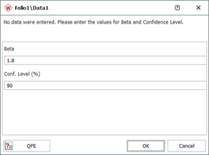
Figure 1: Enter the
value of beta and the confidence level.
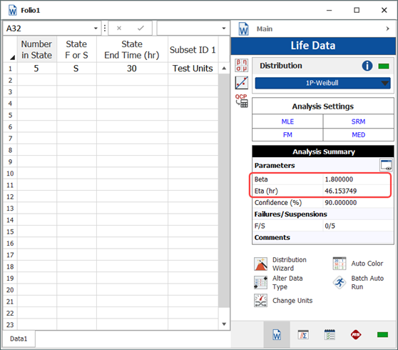
Figure 2: Calculated value of eta.
Case 2: Assume that you have field data from four products and the observation period ended at a different time for each one. Again, no failures were observed. The following table lists the suspension times.
| State (Failure or Suspension) | Time to Failure or Suspension |
| S | 10 |
| S | 18 |
| S | 50 |
| S | 63 |
Because there are four data points with different suspension times, the reliability of each unit is calculated at the end of the observation time. Using the same logic as in Eqn. (1), we have
Substituting the suspension times, the assumed β value, and the confidence level, we get:
We can solve for η as:
![]()
To perform this calculation automatically in Weibull++, enter the data into Weibull++ and select the 1-parameter Weibull distribution. Next, click Calculate. When prompted, enter the value for β and the confidence level and click OK. The value of η is automatically calculated, as shown in Figure 3.
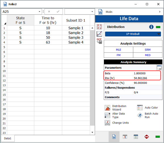
Figure 3: Data set and the calculated value of eta.
Conclusion
In this article, we discussed how the cumulative binomial equation can be used to design an RDT and how it can also be used to estimate the unknown parameter for a data set that contains no failures. The procedure provided in this article is a general guideline; therefore, it can be expanded to other 1-parameter distributions such as exponential, 1-parameter lognormal, 1-parameter Gumbel, etc.
References