Chi-Squared Distribution and Reliability Demonstration Test Design

The Chi-Squared distribution has been widely used in quality and reliability engineering. For instance, it is well-known for testing the goodness-of-fit. In Weibull++, the Chi-Squared distribution is also used for reliability demonstration test design when the failure rate behavior of the product follows an exponential distribution. In this article, we will discuss this feature.

For an exponential distribution, the probability density function (pdf) is:

(1)

where λ is the failure rate. In the case of the exponential distribution, the mean time to failure (MTTF) is the inverse of λ:

(2)

Manufacturers are often required to design a test to demonstrate the MTTF or failure rate of a product. To help engineers with this task, Weibull++ has a built-in tool for design of reliability tests (DRT).

Figure 1: Design of Reliability Tests Tool in Weibull++

In the DRT tool, there are three methods that can be used for reliability demonstration test design: Parametric Binomial, Non-Parametric Binomial and Exponential Chi-Squared. The first two are based on the binomial distribution. From its name, we also can guess that the third method is based on the Chi-Squared distribution and is designed to be used in cases when the failure time distribution is exponential. The reliability function of an exponential distribution is:

(3)

Because of the one-to-one relationship between the failure rate, MTTF, and reliability at time t, the test plan can be designed based on a requirement for either metric. For example, in Figure 1 the required lower bound of MTTF is 100 at a confidence level of 90%. This is the same as requiring the upper bound of the failure rate to be 1/100 = 0.01, or requiring the lower bound of the reliability at time t to be e-0.01xt.

Defining the accumulated test time as T, the following formula is used for calculating T:

or:

(4)

where r is the number of failures and CL is the confidence level.

The above equation is well-known to many engineers nowadays. However, it was not so well-known 15 years ago according to Gorski [1] who wrote: "Well-known to whom? My guess is that less than 0.1% of reliability and quality assurance engineers know it even though many statisticians do. In my 23 years of industry experience I never met an engineer who knew it and yet I worked on projects such as Minuteman I and Apollo where the intent was to bring on board the best people available." To popularize its application, Gorski wrote a paper on the formula and showed how to use it to design a test plan by using a Chi-Squared distribution table. These days, it is not a popular idea to use a table and a hand calculator to design a test plan using Eqn. (4). It is much easier to do the calculation using the DRT tool in Weibull++.

The question now is: why is Eqn. (4) valid? In other words, why can the Chi-Squared distribution be used for design of reliability demonstration tests? In the following discussion, we will provide an explanation.

When the failure times follow an exponential distribution, the number of failures in the time interval T follows a Poisson distribution with associated parameter λT. The relationship is given by:

P(N(T)=i) =

where N(T) is the number of events during time T.

The relationship above can then be used to obtain the upper bound of the failure rate λ by solving the following equation:

1-CL=

(5)

where:

r is the total number of failures.
CL is the confidence level.
λ is the failure rate at confidence level of CL.

We can then manipulate Eqn. (5) in a number of steps so that we can show the relationship with the Chi-Squared distribution.

If we define x = λT, then Eqn. (5) becomes:

(6)

Using Eqn. (6), for a given confidence level CL, the corresponding upper bound of the random variable X can be solved for. The upper bound is x, a realization of X. Eqn. (6) in fact shows the cumulative distribution function for the random variable X. It can be rewritten as:

(7)

Eqn. (7) can then be related to the Gamma distribution. For a Gamma distribution Y~Gamma(k,λ), the cumulative distribution function (cdf) is:

(8)

Comparing Eqn. (7) to Eqn. (8), one can see that x follows the Gamma distribution X ~ Gamma(r+1,1). Based on the properties of a Gamma random variable, we know 2X ~ Gamma(r+1,2). In addition, is a special case of the Gamma distribution if the random variable follows Gamma(r+1,2). Therefore, we can also say 2X ~ . Since x = λT, we know the upper bound of the failure rate is:

(9)

From the relationship between the exponential, Gamma and Chi-Squared distributions, we have shown why the Chi-Squared distribution can be used in design of reliability tests when the units to be tested follow an exponential distribution. Two examples of using Eqn. (9) are given next.

Example 1

An engineer is required to determine the minimal test time in order to demonstrate that the MTTF of a product is at least 500 hours with a confidence level of 90%. The product is known to follow an exponential distribution. Based on the available resources, one failure is allowed in the test. So what should the test time be?

Using Eqn. (9), we get:

So a total of 1944.89 hours of testing is needed. The above calculation can also be done in Weibull++, as shown below.

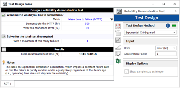
Figure 2: Result for Example 1

Example 2

Assume the failure time of a system follows the exponential distribution. The warranty time of this system is 1000 operating hours. The manufacturer is required to show that the reliability of the system at the 1000th hour is at least 95% with a confidence level of 50%. No failures are allowed in the test. How long should the test last?

Since:

We can get the required MTTF:

By applying the Chi-Squared equation, the required test time, T, can be solved as:

This solution also can be found using Weibull++.

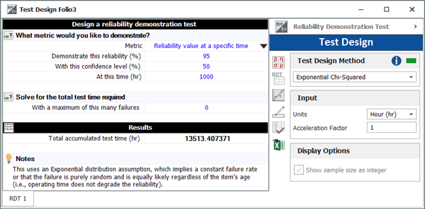
Figure 3: Result for Example 2

Conclusion

The Chi-Squared distribution is successfully used in reliability test designs when the assumption of a constant failure rate is valid. This article explains why the Chi-Squared distribution can be applied by using the relationship between the exponential distribution, the Gamma distribution and the Chi-Squared distribution. Two examples are provided to illustrate the step-by-step calculations. Weibull++ can be used to automate these calculations.

References

[1] Andrew Gorski, "Chi-Squared Probabilities Are Poisson Probabilities in Disguise." IEEE Transactions on Reliability, vol. R-34, No. 3, 1985.