Another Look at the Shape Parameter of the Weibull Distribution (Beta)
[Editor's Note: This article has been updated since its original publication to reflect a more recent version of the software interface.]
It is well known that the shape parameter of the Weibull distribution, beta (β), represents the failure rate behavior. If beta is less than 1, then the failure rate decreases with time; if beta is greater than 1, then the failure rate increases with time. When beta is equal to 1, the failure rate is constant. Assume that we have two failure data sets. From one data set, the estimated beta is 5; from another data set, the estimated beta is 3. Both have increasing failure rates. If the two data sets were combined together, would the estimated beta for the overall data set be a value between 3 and 5, or would it be a value outside of this range? Could it be less than 1, which would imply that the combined data set has a failure rate that is decreasing with time? In the article, we will use examples to show the relationship between these betas.
In order to answer the above questions, we will look at the issue from another perspective. Assume there is the one set of life data that is fitted using a Weibull distribution. This data set has a shape parameter β. If we separate the data into two groups and fit each group with a separate Weibull distribution, we get β1 and β2 as the shape parameters of the two groups. If we suppose that β1 < β2, will β1 < β < β2 always be true, or is there some other relationship between these beta values?
Suppose that a testing engineer obtained the life data shown in Table 1. According to previous experience, the 2-parameter Weibull distribution should be used to fit the data. The analysis using Weibull++ shows that β = 0.9812 and η = 73.6036, as shown in Figure 1.
Table 1: Failure Data
| State (F or S) | Time to State | Item Index |
| F | 2 | 1 |
| S | 3 | 2 |
| F | 5 | 3 |
| S | 7 | 4 |
| F | 11 | 5 |
| S | 13 | 6 |
| S | 17 | 7 |
| S | 19 | 8 |
| F | 23 | 9 |
| F | 29 | 10 |
| S | 31 | 11 |
| F | 37 | 12 |
| S | 41 | 13 |
| F | 43 | 14 |
| S | 47 | 15 |
| S | 53 | 16 |
| F | 59 | 17 |
| S | 61 | 18 |
| S | 69 | 19 |
| F | 75 | 20 |
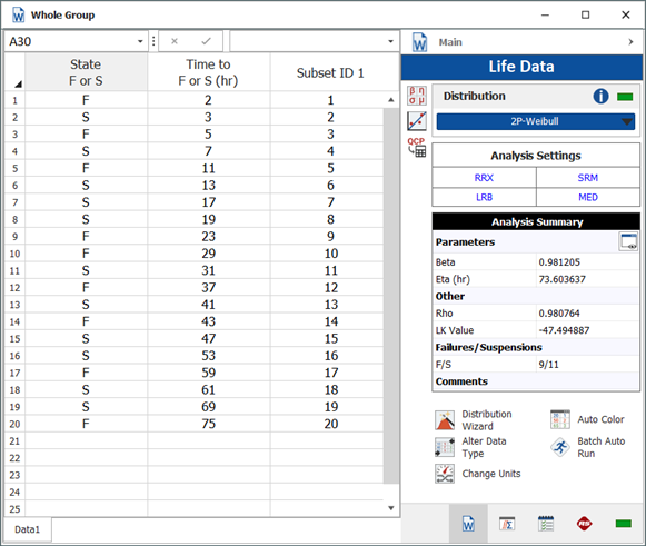
Figure 1: Data Analysis for
the Entire Data Set
To illustrate the subgroups parameters, we extract different subgroups from the full data set. We could use different methods to accomplish this. For the first method, we separate data from the middle point of the entire group. We classify the early failure items as "Subgroup I" and the later failure items as "Subgroup II." These two subgroups are listed in Table 2.
Table 2: Method I Subgroup Data
| Subgroup I (Early) | Subgroup II (Later) | |||
| Item Index |
State (F or S) |
Time to State |
State (F or S) |
Time to State |
| 1 | F | 2 | S | 31 |
| 2 | S | 3 | F | 37 |
| 3 | F | 5 | S | 41 |
| 4 | S | 7 | F | 43 |
| 5 | F | 11 | S | 47 |
| 6 | S | 13 | S | 53 |
| 7 | S | 17 | F | 59 |
| 8 | S | 19 | S | 61 |
| 9 | F | 23 | S | 69 |
| 10 | F | 29 | F | 75 |
The analysis using the 2-parameter Weibull distribution shows that Subgroup I (Early) has β1 = 1.105 and η1 = 24.0872, while Subgroup II (Later) has β2 =3.6717 and η2 = 70.8740.
A second method to extract different subgroups is to separate the data according to the failure index. Entries with odd index numbers are put in Subgroup I and entries with even index numbers are assigned to Subgroup II. These two subgroups are listed in Table 3.
Table 3: Method II Subgroup Data
| Subgroup I (Even) | Subgroup II (Odd) | |||
| Item Index |
State (F or S) |
Time to State |
State (F or S) |
Time to State |
| 1 | S | 3 | F | 2 |
| 2 | S | 7 | F | 5 |
| 3 | S | 13 | F | 11 |
| 4 | S | 19 | S | 17 |
| 5 | F | 29 | F | 23 |
| 6 | F | 37 | S | 31 |
| 7 | F | 43 | S | 41 |
| 8 | S | 53 | S | 47 |
| 9 | S | 61 | F | 59 |
| 10 | F | 75 | S | 69 |
The analysis using the 2-parameter Weibull distribution shows that Subgroup I (Odd) has β1' = 0.7419 and η1' = 62.4596, while Subgroup II (Even) has β2' =2.4834 and η2' = 61.4978.
As we can see, for the first method, β < β1 < β2, and for the second method, β1' < β < β2'. So it depends on how the subgroup was extracted from the original data. From the above examples we also can see that there is no fixed relationship between these betas.
Now let’s examine the definition of the standard deviation of the Weibull distribution:
where
![]() is the gamma
function evaluated at the value of
is the gamma
function evaluated at the value of
 .
.
Table 4 lists the standard deviation values for the overall group and for each subgroup.
Table 4: Distribution Parameters for Different Subgroups
| Whole Group |
Subgroup Early |
Subgroup Later |
Subgroup Odd |
Subgroup Even |
|
| β | 0.981 | 1.105 | 3.6717 | 0.7419 | 2.4834 |
| η | 73.6036 | 24.0872 | 70.8740 | 62.4596 | 61.4978 |
| 1/β | 1.0941 | 0.9050 | 0.2724 | 1.3479 | 0.4027 |
| σT (standard deviation) | 75.63642 | 21.0307 | 19.3781 | 102.75802 | 23.4846 |
We can see that the relationship between the 1/β of the whole group and each of the subgroups are similar to the relationships of their standard deviations σT. In other words, 1/β roughly reflects the standard deviation of the distribution. For example, in our first classification method I, as 1/β for the whole group is greater than either subgroup; so is its σT is greater than either subgroup.
It will be even clearer if we use the logarithmic transformation of the raw data to fit
a Gumbel distribution. As we know, the logarithm transform of Weibull data follows
the Gumbel distribution with μ = ln(η) and
![]() , where μ is the
location parameter and σ is the scale parameter of the Gumbel distribution. The
standard deviation for the Gumbel distribution is given by:
, where μ is the
location parameter and σ is the scale parameter of the Gumbel distribution. The
standard deviation for the Gumbel distribution is given by:
![]()
From the above equation, we can see how 1/β reflects the spread of a data set.
Conclusions
In this article, we answered the question about the relationship between the beta for the entire data set and the betas for subgroups of that data set. As we can see, this relationship is not fixed, and can change. Moreover, 1/β can be interpreted as something similar to the standard deviation of a data set. So 1/β not only represents the behavior of the failure rate, it also reflects the spread of a data set.