Unbiasing Parameters in Weibull++

[Editor's Note: This article has been updated since its original publication to reflect a more recent version of the software interface.]

Commonly used methods for parameter estimation, such as the maximum likelihood estimation (MLE) and the least squares estimation (LSE) or rank regression (RR), are known to be biased. This is particularly true with small sample sizes and censored data. Bias correction methods have been studied in the literature. A well known example is the standard deviation obtained using MLE for which it can be shown that an unbiased estimator may be obtained [1, 2]. Weibull++ makes it possible to calculate unbiased parameters for the standard deviation in the Normal distribution, and for beta in the 2-parameter Weibull distribution. In this article, we will discuss the method used in Weibull++ to calculate the unbiased beta estimator for MLE, for both complete and censored data. Unlike the case of the Normal distribution, this is an empirical method obtained via simulation [3].

Unbiased and Biased Estimators

If the mean value of an estimator equals the true value of the quantity it estimates, then the estimator is called an unbiased estimator. For example, assume that the sample mean is being used to estimate the mean of a population. Using the Central Limit Theorem, the mean value of the sample means equals the population mean. Therefore, the sample mean is an unbiased estimator of the population mean.

If the mean value of an estimator is either less than or greater than the true value of the quantity it estimates, then the estimator is called a biased estimator. For example, suppose you decide to choose the smallest observation in a sample to be the estimator of the population mean. Such an estimator would be biased because the average of the values of this estimator would always be less than the true population mean. In other words, the mean of the sampling distribution of this estimator would be less than the true value of the population mean it is trying to estimate. Consequently, the estimator is a biased estimator.

Obtaining the Unbiased Beta

The method used in Weibull++ for obtaining the unbiased estimator of beta is described in detail in [3]. The general steps are summarized below.

Step 1: A bias correcting factor is defined such that:

(1)

where:

• bβ is the biased estimator of β (obtained with MLE or RR).
• bU is the unbiased estimator of β.
• U is the correcting factor.

Step 2: A correcting factor model that is a function of the sample size is assumed.

Step 3: Using Monte Carlo simulation, data sets with different sample size are generated. Note that by doing this, the true parameters of the distribution are known.

Step 4: Using unconstrained linear optimization, parameters for the correcting factor model are obtained such that the square error between the known parameter of beta and the unbiased estimator is minimized.

In the case of data sets with right censored data, a model that is a function of both the sample size and the censoring level is selected and data sets are generated varying both the sample size and the censoring level.

Weibull 2-Parameter MLE Solution

Data Sets Without Right Censored Data (No Suspensions)

When dealing with data sets with no suspensions, the following model is used:

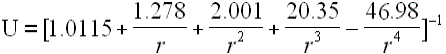
(2)

where r is the number of failures (includes interval and left censored data).

The unbiased estimator of β can be obtained as follows.

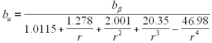
(3)

Data Sets with Right Censored Data (Suspensions)

When dealing with data sets with suspensions, the following model is used:

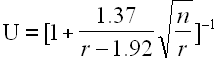
(4)

where:

• r is the number of failures (includes interval and left censored data).
• n is the total sample size.

The unbiased estimator of β can be obtained as follows.

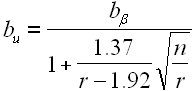
(5)

Obtaining Eta

Once the unbiased estimator of beta has been obtained, eta is solved for. This is equivalent to using Weibull++'s, "Alter One Parameter" feature, with the newly found beta to solve for eta.

Example with Complete Data

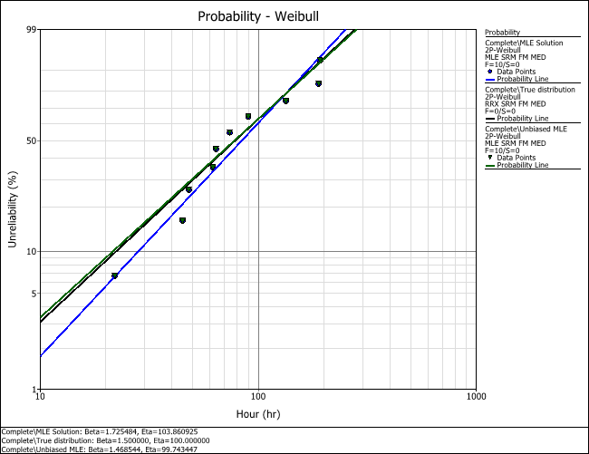
Ten data points have been generated using a Weibull distribution with beta = 1.5 and eta = 100. The following failures are recorded: 22, 45, 48, 62, 64, 74, 90, 134, 189 and 192.

After estimating the parameters with MLE, we obtain a beta of 1.7255 and an eta of 103.8609. We can then calculate the new unbiased beta using Eqn. (3), to obtain a beta of 1.4689.

We can alter beta to recalculate eta by choosing Life Data > Options > Alter One Parameter (and Recalculate) > Alter Beta.

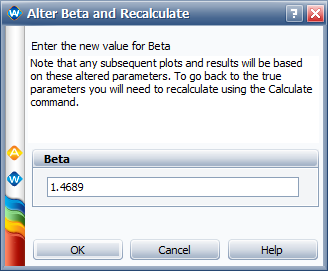
After recalculating, eta is now 99.7492.

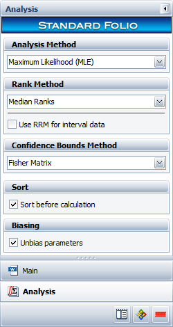
We can do this automatically in Weibull++ by selecting Unbias parameters from the Analysis page of the control panel. Note that this option is only available for the Weibull 2-parameter distribution and when MLE has been selected as the estimation method.

The plot shows the true probability line (black), the MLE solution line (blue) and the unbiased parameters line (green).

Example with Suspended Data

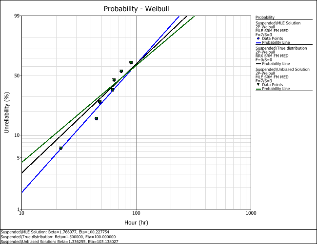
Assume that we will suspend all failures that occurred after 120 in the previous example. The following failures are recorded: 22, 45, 48, 62, 64, 74 and 90. The other 3 data points are suspended at 120.

After estimating the parameters with MLE, we obtain a beta of 1.7670 and an eta of 100.2278. We can then calculate the new unbiased beta using Eqn. (5), to obtain a beta of 1.3363.

We can alter beta to recalculate eta by using the Alter One Parameter (and Recalculate) command. After recalculating, eta is now 103.1375.

The plot shows the true probability line (black), the MLE solution line (blue) and the unbiased parameters line (green).

Conclusion

In this article, we presented the methods used in Weibull++ to unbias parameters for the 2-parameter Weibull distribution, when using MLE solutions. Two different correcting factor formulas are used depending on whether the data set is complete or has censoring. In the examples presented, both unbiased lines were closer to the true value than using the MLE solutions. Keep in mind that this may not be true for every sample. However, if the experiments presented were to be repeated a number of times, the average unbiased beta of all these experiments is expected to be closer to the true value than the average beta of the MLE solutions.

References

[1] ReliaSoft Corporation, Life Data Analysis Reference, Tucson, AZ: ReliaSoft Publishing, 2005.

[2] Dietrich, D., SIE 530 Engineering Statistics Lecture Notes. The University of Arizona, Tucson, AZ.

[3] L.F. Zhang, M. Xie, L.C. Tang, "Bias correction for the least squares estimator of Weibull shape parameter with complete and censored data," Reliability Engineering and System Safety, vol. 91, pp. 930–939, 2006.