Comparison of Fisher Matrix and Likelihood Ratio Confidence Bound Methods
[Editor's Note: This article has been updated since its original publication to reflect a more recent version of the software interface.]
In Weibull++, there are several ways to calculate reliability confidence bounds for different distributions. The Fisher matrix (FM) method and the likelihood ratio bounds (LRB) method are both used very often. Both methods are derived from the fact that the parameters estimated are computed using the maximum likelihood estimation (MLE) method. However, they are based on different theories. The MLE estimates are based on large sample normal theory, and are easy to compute. However, when there are only a few failures, the large sample normal theory is not very accurate. Thus, the FM bounds interval could be very different from the true values.[1] The LRB method is based on the Chi-Squared distribution assumption. It is generally better than FM bounds when the sample size is small. In this article, we will compare these two methods for different sample sizes using the Weibull distribution.
Fisher Matrix Confidence Bounds
The bounds are calculated using the Fisher information matrix. The inverse of the Fisher information matrix yields the variance-covariance matrix, which provides the variance of the parameters.[2] The bounds on the parameters are then calculated using the following equations:
![]()
where:
- E(G) is the estimate of the mean value of the parameter G.
- Var(G) is the variance of the parameter G.
- α = 1 - CL, where CL is the confidence level.
- za is the standard normal statistic.
The bounds for functions of the distribution parameters (e.g., the reliability and the unreliability) also can be calculated using the above equation. For example, the variance of the reliability can be estimated from the variance/covariance matrix of the distribution parameters.
Likelihood Ratio Confidence Bounds
The likelihood ratio bounds method is often preferred over the Fisher Matrix confidence bound method in situations where there are smaller sample sizes. For data sets with a larger number of data points, there is no significant difference in the results of these two methods. Likelihood ratio bounds are calculated using the likelihood function as follows:
where:
- L(G) is the likelihood function for the unknown parameter G.
 is the likelihood function calculated at the estimated
parameter value
G.
is the likelihood function calculated at the estimated
parameter value
G.- α = 1 - CL, where CL is the confidence level.
-
 is the Chi-Squared statistic
with
k degrees of freedom, where
k is the number of quantities jointly
estimated.
is the Chi-Squared statistic
with
k degrees of freedom, where
k is the number of quantities jointly
estimated.
Similarly, the bounds of the reliability also can be calculated based on the Chi-Squared distribution.[3]
Comparison of the FM and LRB Methods
To illustrate the difference, we will compare the confidence bounds over time with a fixed BX% using three data sets. We use sample sizes of 5, 50 and 100 with the settings shown in the following table.
Table 1: Sample Settings
| Confidence Bound Method | FM Method | LRB Method |
| BX | 5 | 5 |
| Confidence Bound used | 1 sided | 1 sided |
| Confidence Level | 0.9 | 0.9 |
| Weibull 2P | Beta=0.5, Eta=20 | Beta=0.5, Eta=20 |
First we create a data set with a sample size of 5 data points using the Monte Carlo tool from Weibull++, as shown next.
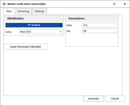
Figure 1: Use Monte Carlo to generate
sample
The generated data set is shown next.
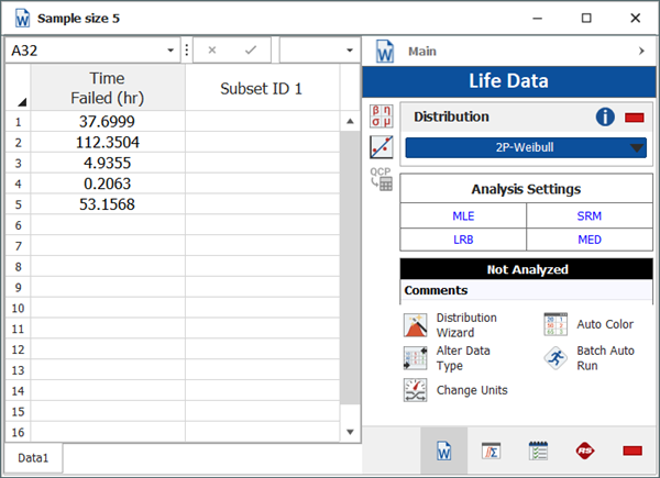
Figure 2: Generated data set for a
sample size of 5
On the Analysis tab, choose Maximum Likelihood (MLE) for the Analysis Method, and Use Likelihood Ratio as the Confidence Bound Method. Leave all other options with the default values and then click the Calculate button.
Using the QCP tool we can calculate the upper and lower confidence bounds. For this example, choose Both One Sided on the Confidence Bounds tab and then go to the Basic Calculations tab and choose BX Information and type "5" in the input box to reflect a 5% probability of failure. Click Calculate. The results are shown next.
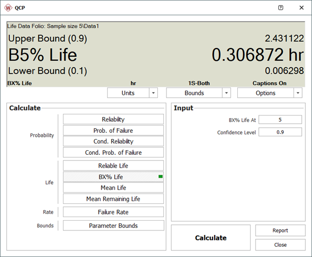
Figure 3: QCP result with LRB method
In the Analysis tab, if you choose Use Fisher Matrix bounds for the Confidence Bounds Method, you get similar results for the time confidence bounds at B5. Table 2 illustrates the results for the two different methods.
Table 2: Comparison of FM and LRB methods and simulation results for a sample size of 5
| FM Method | LRB Method | Simulation Results | |
| Upper Bound | 4.7155 | 2.4311 | 2.028566221 |
| Time | 0.3069 | 0.3069 | 0.144772350 |
| Lower Bound | 0.02 | 0.0063 | 0.004437272 |
| Confidence | 1S @0.9 | 1S @0.9 | 1S @0.9 |
| Bound Width | 4.6955 | 2.4248 | 2.024128949 |
| Bound Ratio | 235.775 | 385.8888889 | 457.1651593 |
The simulation results in Table 2 were obtained from SimuMatic with the following settings.
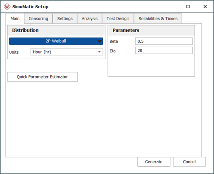
Figure 4: SimuMatic Setup window
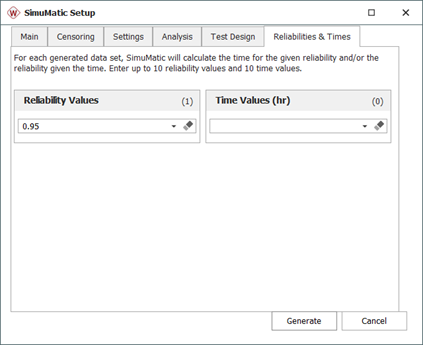
Figure 5: SimuMatic Setup for a data
sample size of 5
SimuMatic generated 1,000 data sets for this example. The beta and eta of the Weibull distribution for each of the 1,000 data sets were estimated using the MLE method. From the 1,000 paired beta and eta parameters, 1,000 B5 values were also calculated. To obtain the 1-sided 90% confidence bounds, these 1,000 B5 values first need to be sorted in ascending order. The 100th value will be the lower bound and the 900th value will be the upper bound. Since there are no assumptions in obtaining the simulation bounds, the results serve as the benchmark for evaluating confidence bound estimation methods.
In Table 2, bound width and bound ratio are calculated using the following formulas:
bound width = upper bound – lower bound
bound ratio = upper bound/lower bound
As we can see, the LRB bound width is narrower than the FM bound width, and the LRB bound ratio is higher than the FM bound ratio. Using the simulation results obtained with SimuMatic, the comparison shows that the LRB result is much closer to the simulation result than the FM result is.
Repeating the above procedures for sample sizes of 50 and 100, we get similar comparisons, which are shown in Tables 3 and 4.
Table 3: Comparison of FM and LRB methods and simulation results for a sample size of 50
| Fisher Matrix Method | Likelihood Ratio Method | Simulation Results | |
| Upper bound | 0.2407 | 0.2217 | 0.1518388385 |
| Time | 0.0923 | 0.0923 | 0.05481979463 |
| Lower bound | 0.0354 | 0.0321 | 0.0184973181 |
| Confidence | 1S @ 0.9 | 1S @0.9 | 1S @0.9 |
| Bound Width | 0.2053 | 0.1896 | 0.13334152 |
| Bound Ratio | 6.7994 | 6.9065 | 8.208694778 |
Table 4: Comparison of FM and LRB methods and simulation results for a sample size of 100
| Fisher Matrix Method | Likelihood Ratio Method | Simulation Results | |
| Upper bound | 0.1659 | 0.1593 | 0.109948402 |
| Time | 0.086 | 0.086 | 0.055857738 |
| Lower bound | 0.0446 | 0.0426 | 0.024601808 |
| Confidence | 1S @ 0.9 | 1S @0.9 | 1S @0.9 |
| Bound Width | 0.1213 | 0.1167 | 0.085346594 |
| Bound Ratio | 3.7197 | 3.7394 | 4.469118774 |
With the increase in sample size, the difference between the FM and LRB bound widths gets smaller, and both get very close to the simulation bound width and bound ratios. This supports our statement in the introduction that the LRB method usually is more accurate than the FM bound for small sample sizes, and there is not much difference between the two methods if sample size is large enough.
References
[1] Scott
A. Vander Wiel, William Q. Meeker, "Accuracy of Approximate
Confidence Bounds Using Censored Weibull Regression Data
from Accelerated Life Tests," IEEE Transactions on Reliability,
Vol. 39, No. 3, 1990, August.
[2] ReliaSoft Corporation.
"Individual and Joint Parameter Bounds in Weibull++."
Reliability Hotwire Issue 101. 2009.
[3] ReliaSoft Corporation, Life Data Analysis Reference,
Tucson, AZ: ReliaSoft Publishing, 2007.