A Pro-rata Warranty Model for Non-Repairable Products
In the current consumer market, a product’s warranty is one of the important factors in the consumer’s decision-making process. From vehicles to home appliances, when several products perform similar functions, customers usually prefer to purchase the product that provides the better warranty. In this article, we will discuss several warranty policies. One example will be given for calculating the predicted warranty cost.
A warranty is a contract or an agreement under which the manufacturer of a product or service must agree to repair, replace or provide service when the product fails or the service does not meet the customer’s requirement before a specified time (warranty length) [1]. There are three commonly-used warranty policies: the ordinary free replacement warranty, the unlimited free replacement warranty and the pro-rata warranty.
Ordinary Free Replacement Warranty: Under this warranty, if a product fails before the end of the warranty period because of quality or reliability issues, it will be replaced or repaired at no cost to the customer. The repaired product is then covered by an ordinary free replacement warranty. The length of the warranty for the repaired product is equal to the remaining length of the original warranty. The ordinary free warranty is used by many vehicle and home appliance companies.
Unlimited Free Replacement Warranty: Under this warranty, if a product fails before the end of the warranty period, it will be replaced or repaired at no cost to the customer. The repaired product is then covered by a new unlimited free replacement warranty. The length of the new warranty is equal to the length of the original one. The unlimited free replacement warranty is used for small electronic appliances that have high early failure rates. The length of the unlimited free replacement warranty usually is short.
Pro-rata Warranty: Under this warranty, if an item fails before the end of the warranty period, it is replaced at a cost that depends on the age of the item at the time of failure. The replacement item is then covered by an identical new warranty. This type of warranty sometimes is also called partial warranty, since only a part of the initial cost is covered. It is usually used for non-repairable items such as tires and batteries.
If a product is covered by a warranty, the manufacturers need to decide the length of the warranty and predict the warranty cost. Sometimes the warranty length is affected by the competitors on the market. For example, no one will buy a new car with only a 1 year limited warranty since many cars are covered by 5, 7 or even 10 year warranty assurances. Once the warranty policy has been decided, the amount of capital that must be allocated to cover the future warranty cost needs to be predicted. In the following section, we use an example to illustrate how to predict the warranty cost for the pro-rata warranty policy.
Example
A pro-rata warranty is applied to a product. Assume that the unit price before adding the warranty cost is $50 and the warranty length is five years or 1825 days. It is also known that the failure time distribution is a Weibull distribution with a shape parameter of 1.2 and a scale parameter of 5,600 days. What should be the unit price in order to cover the warranty cost?
Let’s define the following variables:
- c': unit price before adding the warranty cost
- r: expected warranty cost per unit
- c: unit price after adding the warranty cost, c = c’ + r
- N(t): number of failure at time t
- L: product lot size for warranty cost determination
- w: duration of the warranty period
- C(t): pro-rata customer cost at time t, C(t)=c[1-(t/w)]
- Tc: total warranty cost of a lot of size L
The probability density function (pdf) for a Weibull distribution is [2]:

and the cumulative distribution function (cdf) is:

The expected number of failures
for the whole lot by time t is:
![]() .
.
The total number of failures in
the interval from t to t+dt is:
![]() .
.
The expected total cost for the
failures from t to t+dt is:
![]() .
.
So, the total expected cost for the warranty period is:

The warranty cost per unit is:

For this example:
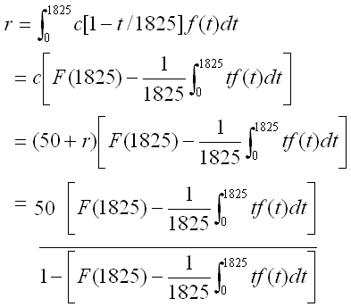
From the above equation, we can solve for the warranty cost per unit r = 6.117. For the integral, a mathematic software package such as MathCAD can be used to get the result.
Therefore, to cover the warranty cost, the price per unit should be:
![]()
If the lot size is 10,000, the estimated warranty cost will be $61,170. For different warranty lengths, the calculated unit price is given in the following table.
| Warranty Length (Year) | Unit Price ($) |
| 2.00 | 51.99 |
| 2.50 | 52.64 |
| 3.00 | 53.27 |
| 3.50 | 53.94 |
| 4.00 | 54.65 |
| 4.50 | 55.37 |
| 5.00 | 56.12 |
| 5.50 | 56.89 |
| 6.00 | 57.67 |
| 6.50 | 58.48 |
| 7.00 | 59.30 |
| 7.50 | 60.15 |
| 8.00 | 61.01 |
| 8.50 | 61.89 |
| 9.00 | 62.78 |
| 9.50 | 63.69 |
| 10.00 | 64.62 |
This is also shown in the following figure.
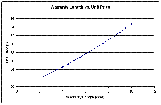
Figure 1: Unit Price for Different Warranty Lengths
If customers will not buy the product for more than $60, then the warranty length should not be longer than 7 years.
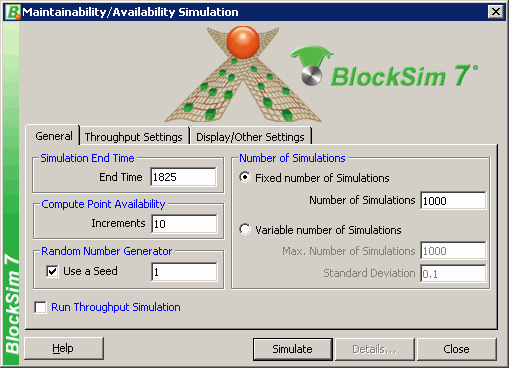
The above example also can be solved using simulation. You can use ReliaSoft's RENO, Weibull++ or BlockSim software to obtain the desired results. The following steps will show how to estimate the warranty cost in BlockSim.
First, create a block with the following settings:

Second, conduct the simulation with the End Time = 1825.
Make sure you save the simulation results by selecting Save Log of Simulations on the Display/Other Settings page, as shown next.

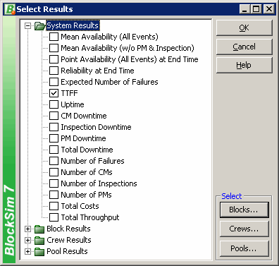
Click Select Results to save the Time to the First Failure (TTFF).
The saved failure times will look like the file shown next.
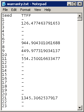
For each simulation run (the seed column), you can calculate the pro-rata time using 1 - ti /1825. If the item fails, ti is the failure time. Otherwise, it is the suspension time 1825.
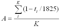
where K is the number of simulations and A denotes the entire equation. As the number of simulations increases, the value of A approaches the analytical solution:
![]()
Using the above simulation settings, we get A = 0.115, while the analytical solution is 0.109. The warranty cost per unit is calculated by:

Solving the above equation, we get r = 6.497. The unit price for the product after adding the warranty cost is $56.497, which is very close to the analytical solution of $56.117.
Conclusion
In this article, we discussed three common kinds of warranty policies, which are typically used for different types of products. We used an example to calculate the expected warranty cost for a pro-rata warranty policy and we provided both analytical and and simulation results. The analytical solution requires solving a complex integral, so it can be cumbersome for engineers to use. Simulation is a simple and easy method for calculating warranty costs that can provide relatively accurate results. Note that the ordinary free replacement warranty policy and the unlimited free replacement warranty policy are quite simple and also can be easily modeled in BlockSim.
References
[1] Elsayed, E. A. Reliability Engineering, Massachusetts: Addison Wesley, 1996.
[2] ReliaSoft Corporation, Life Data Analysis Reference, Tucson, AZ: ReliaSoft Publishing, 2007.